Contents
How to Generate a SurfaceThe Surface Display Object Interface
Surface Preferences
Electrostatic Surfaces
Charge Assignment
Background Theory
 |
CCP4 Molecular Graphics Documentation | |
| Molecular Surfaces |
| Documentation Contents | On-line Documentation | Tutorials | CCP4mg Home |
To generate a molecular surface you must first load the molecule.
The molecule will then be listed in the Display Table window with one
model display object line showing the atom selection, colour and style
for the displayed model.
To create a surface you :
Create a new Surface display object.
To do this click on the icon menu of the
model object (the dot next to the molecule name) and select Add display object
and then Surface.
In the display table the first column for the surface display object are
Atom Selection and the third is Colour (note how this is different from model display objects).
The second column is for selection of context atoms.
Note that the surface is not drawn immediately; you need to click on the surface icon
and select Show from from menu.
The selection interface is identical to the selection interface for model display objects.
The most useful options are probably All peptide to create a surface
over the protein and Neighbourhood which allows you to select just the area
of the protein around a given residue or ligand.
Beware that if you select a limited number of atoms then the surface will probably
wrap around the back of the selected atoms.
To prevent this you should set the context selection (in the third column) appropriately. The most useful context selection option, to use when you have selected a limited set of atoms in the protein, is All peptide. The surface calculation algorithm will automatically exclude hydrogen atoms and atoms closer than 0.1A. Also if the input set has atoms with more than one alternate location then only the atoms with the first alternate location are used.
The Colour menu has the same options as the model colour menu with the additional
options to colour by Electrostatic potential and by Potential from map.
The electrostatic potential is calculated on demand, beware this is a slow process.
The colouring scheme for electrostatic potential surfaces and map surfaces can be changed using the option on the icon menu to Change colouring.
The surface display object icon menu (click on ![]() ) has options:
) has options:
The Atom selection and Colour scheme menus are the same as for model display objects except there is an option for colouring by Electrostatic potential.
The middle menu on the display table menu is to select the atoms that provide the context for drawing the surface. By default this context is Same as selection. To draw a surface that, for example, covers just the residues of a ligand binding site the selection should be set to the neighbourhood of the ligand and the context should be All peptide. This context menu has a subset of the usual selection interface.
The Preferences window can be opened from the Tools pull-down menu and the folder Sufaces contains a Surface Parameters option. Alternatively preferences to apply to only one surface can be accessed by clicking Surface drawing options.. on the surface icon menu(![]() ). The variable parameters are:
). The variable parameters are:
Surface probe radius (0-3) is the radius of the probe atom which is considered to be rolling over the surface of the molecule. A value of 1.5 Å, corresponding to a water molecule, is normally used. Note that reducing this value to zero is effectively the same (but less efficient!) as drawing the model with display style Spheres.
Cutoff distance for context atoms After the user has selected a set of atoms to be surfaced and, optionally, a set of context atoms, the algorithm excludes any context atoms more than this cutoff distance from the set of surface atoms. This can speed up the calculation and only in the case on a very large prone radius might it be necessary to increase this value.
Resolution in degrees This is the maximum arc angle for any triangular facet on the surface. The default value of 30degrees gives a reasonably fast calculation time. For quality output images, particularly close-up of the surface, it may help to reduce this to 5-10degrees.
Blend colour borders By default each triangular facet of the surface is assigned to one or other of the underlying atoms and is coloured the same as the underlying atom. If this option is switched on then a triangle may straddle between two atoms so that, if the two atoms are different colours, the colours are blended across the triangle. This helps to reduce the jaggedness of colour edges when seen close up but should be used in conjunction with small values for the resolution.
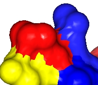 |
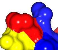 |  |
Resolution=30, |
Resolution=10, |
Resolution=10, |
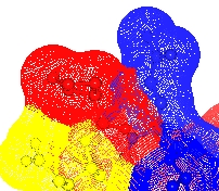
Maximum dot separation Set the maximum separation of dots on the surface.
Dot size is the size of the dot in pixels. Whether non-integer values are interpreted (by anti-aliasing the edge of the dot) seems to depend on the graphics capability of the machine.
Note that there are limits set on some of the above parameters: the range is indicated on the interface. If you want to change these values contact CCP4mg developers for advice.
The electrostatic potential in CCP4mg is in units of Volts. This is different from GRASP for which potentials are in kT/e (25.6mV, 0.593 kcal/mole at 25oC). To convert CCP4mg values to GRASP values multiple by 0.0256.
By default the charges used in the calculation are taken from the file ccp4mg/data/ener_lib.cif. This file lists attributes such as hydrogen-bonding capability and van Der Waals radius for the atom energy types. The file is in mmCIF format with a loop for the atom energy types (called _lib_atom) which has an attribute surface_potential_charge. At the time of writing the loop definition and some of the data for nitrogen energy types looks like this
loop_
_lib_atom.type
_lib_atom.weight
_lib_atom.hb_type
_lib_atom.vdw_radius
_lib_atom.vdwh_radius
_lib_atom.ion_radius
_lib_atom.element
_lib_atom.valency
_lib_atom.sp
_lib_atom.surface_potential_charge
..
..
..
NC1     14.00670  D     1.550     1.600    1.32   N   3  2  0.0
NH1     14.00670  D     1.550     1.600    1.32   N   3  2  0.0
NC2     14.00670  D     1.550     1.600    1.32   N   3  2  0.5
NH2     14.00670  D     1.550     1.600    1.32   N   3  2  0.0
NC3     14.00670  D     1.550     1.600    1.32   N   3  2  0.0
So the energy type NC2 has the surface potential charge 0.5 but all other listed energy types have zero surface potential charge.
The atom energy type is defined in the monomer library files which are ccp4mg/data/monomer_library/x/XXX.cif for the residue type XXX. See the atom typing documentation.
Charges specified in the PDB file will over-ride those assigned according to atom energy type. The charge should be in columns 79-80 of the file (i.e. immediately after the atom element type). Atoms in the PDB without assigned charged will be assigned charge according to the atom energy type. If you want to force the charge to be 0.0 then it is necessary to enter a value of 99 in the charge columns of the PDB file.
To see the charge values used in the calculation click on a model display icon menu
 and select Label text and click on the display of charges and click off the display of any other parameters. Then select Label atoms and All atoms from the model display icon menu. Only the atoms with non-zero charge values will be labelled. The charges are assigned to atoms the first time that an electrostatic potential is calculated and before that the labelled charges will reflect the charge values in the PDB file.
It is also possible to list the charged atoms. From the model icon menu select Structure definition and List charges.
Note that there may also be a partial charge labelled _chem_comp_atom.partial_charge in the monomer library files. This data is intended for use in empirical energy calculations (e.g. REFMAC5) and is not used by the electrostatic surface calculation.
The surface is a Lee and Richards surface which is derived (conceptually at least) by rolling a ball which is equivalent to a solvent molecule over the surface of the protein and taking the path of the centre of the ball for the surface. The resultant surface glides over small invaginations in the van der Waals surface of the protein and so, more acturately, represents the volume that is inaccessible to a solvent molecule.
Atom charges are assigned based on a residue lookup table assuming physiological pH, without consideration to synergistic effects. Atom charge is represented as smooth charge density sampled at grid points. Initial grid charges are assigned based on atom charge and atom volume to each grid point inside the atom sphere. The initial discrete charge density is smoothed using charge anti aliasing to reduce grid position artefacts [Bruccoleri, Novotny, Davis, Sharp, 1996].
A solvent envelope of the protein is calculated based on a fast Fourier surface algorithm (insert blurp about the fft algorithm here....). The spatially varying dielectric grid is assigned values between 78 (bulk solvent) and 2 (fully inside the molecule) using volume filtering based this envelope and using harmonic averaging over the nearest nine grid points. Together with charge anti aliasing this approach has been shown to minimize positional artefacts [Bruccoleri, Novotny, Davis, Sharp, 1996].
Solvent screening is modelled as simple Debey-Huckel screening parameter grid, calculated as function of ionic strength of bulk solvent and temperature [Nicholls, Honig 1990]. Default values for ionic strength and temperature are given 150mM and RT respectively.
Using charge, dielectric and Debey-Huckel grids defined in this way, the linearized Poisson boltzmann equation (LPBE) is solved using a finite difference approach. The PBE finite difference matrix is solved iteratively by optimized successive overrelaxation algorithm (SOR) taking advantage of Chebyshev acceleration and odd-even ordering [Davis, McCammon 1988].
The optimized overrelaxation factor is calculated using the spectral radius for LPB matrix approximated as a function of the matrix dimensions.
Computational analyses of the surface properties of protein-protein interfaces. J. Gruber, A. Zawaira, R. Saunders, C. P. Barrett and M. E. M. Noble. Acta Cryst. (2007). D63, 50-57
The interpretation of protein structures: estimation of static accessibility. Lee B, Richards FM. (1971). J Mol Biol 55(3):379-400.