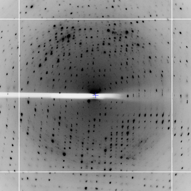
Figure 2: Illustration of the central region of a diffraction pattern from the
example data set.
If you don’t like reading manuals and just want to get started, try:
or
(remembering of course -atom X if you want anomalous pairs separating in scaling.) If this appears to do something sensible then you may well be home and dry. Some critical options:
If this doesn’t hit the spot, you’ll need to read the rest of the document.
In a nutshell, xia2 is an expert system to perform X-ray diffraction data processing on your behalf, using your software with little or no input from you. It will correctly handle multi-pass, multi-wavelength data sets as described later but crucially it is not a data processing package. Specifically, if you use xia2 in published work please include the references for the programs it has used, which are printed at the end of the output.
The system was initially written to support remote access to synchrotron facilities, however it may prove useful to anyone using MX, for example:
The last of these may be most useful for users in a pharmacutical setting, or people wishing to test or benchmark equipment, for example beamline scientists. In all cases however the usage of the program is the same.
Users of macromolecular crystallography (MX) are well served in terms of data reduction software, with packages such as HKL2000, Mosflm1, XDS2 and d*TREK often available and commonly used. In the main, however, these programs require that the user makes sensible decisions about the data analysis to ensure that a useful result is reached. This manual describes a package, xia2, which makes use of some of the aforementioned software to reduce diffraction data automatically from images to scaled intensities and structure factor amplitudes, with no user input.
In 2005, when the xia2 project was initiated as part of the UK BBSRC e-Science project e-HTPX, multi-core machines were just becoming common, detectors were getting faster and synchrotron beamlines were becoming brighter. Against this background the downstream analysis (e.g. structure solution and refinement) was streamlined and the level of expertise needed to use MX as a technique was reducing. At the same time mature software packages such as Mosflm, Scala3, CCP44 and XDS were available and a new synchrotron facility was being built in the UK. The ground was therefore fertile for for the development of automated data reduction tools. Most crucially, however, the author was told that this was impossible and a waste of time - sufficient motivation for anyone.
Without the trusted and capable packages Mosflm, CCP4, Scala and XDS it would clearly be impossible to develop xia2. The author would therefore like to thank Andrew Leslie, Harry Powell, Phil Evans, Wolfgang Kabsch and Kay Diederichs for their assistance in using their programs and modifications they have made. In addition, more recent developments such as Labelit 5, Pointless6 and CCTBX7 have made the development of xia2 much more straightforward and the end product more reliable. The author would therefore like to additionally thank Nick Sauter and Ralf Grosse-Kunstleve for their help.
Development of a package such as this is impossible without test data, for which the author would like to thank numerous users, particularly the Joint Center for Structural Genomics, for publishing the majority of their raw diffraction data.
During the course of xia2 development the project has been supported by the UK BBSRC through the e-HTPX project, the EU Framework 6 through the BioXHit project and most recently by Diamond Light Source. The software itself is open source, distributed under a BSD licence, but relies on the user having correctly configured and licenced the necessary data analysis software, the details of which will be discussed shortly.
As mentioned in the quick start section, to get started simply run:
or
The program is used from the command-line; there is no GUI. The four most important command-line options are as follows:
| Option | Usage |
| -atom X | tell xia2 to separate anomalous pairs i.e. I(+)≠I(-) in scaling |
| -2d | tell xia2 to use MOSFLM and SCALA |
| -3d | tell xia2 to use XDS and XSCALE |
| -3dii | tell xia2 to use XDS and XSCALE, indexing with peaks found from all images |
These specify in the broadest possible terms to the program the manner in which you would like the processing performed. The program will then read all of the image headers found in /here/are/my/data to organise the data, first into sweeps, then into wavelengths, before assigning all of these wavelengths to a crystal.
The data from the experiment is understood as follows. The SWEEP, which corresponds to one “scan,” is the basic unit of indexing and integration. These are contained by WAVELENGTH objects which correspond to CCP4 MTZ datasets, and will ultimately have unique Miller indices. For example, a low and high dose pass will be merged together. A CRYSTAL however contains all of the data from the experiment and is the basic unit of data for scaling. This description of the experiment is written automatically to an instruction file, an example of which is shown in Figure 1
The most straightforward way to discuss the operation of the program is through demonstrations with real examples. The first of these is a dataset from a DNA / ligand complex recorded at Diamond Light Source as part of ongoing research. The structure includes barium which may be used for phasing, and the data were recorded as a single sweep. As may be seen from Figure 2, the quality of diffraction was not ideal, and radiation damage was an issue. Initially the data were processed with
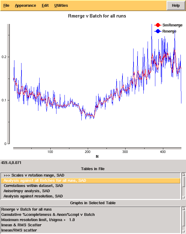
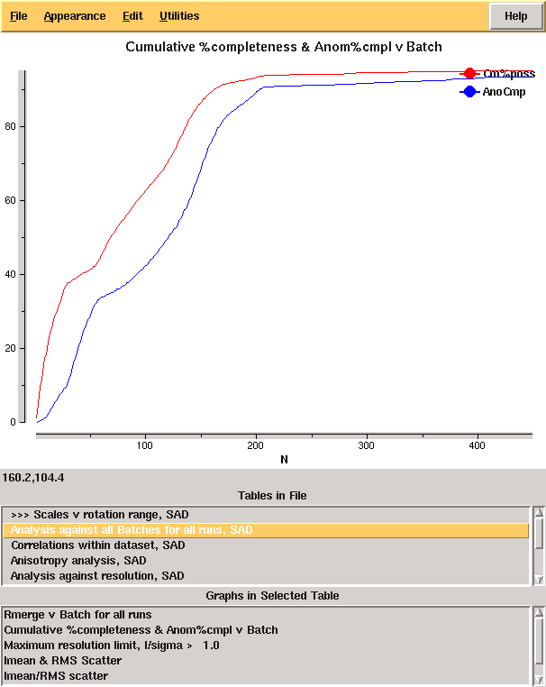
giving the merging statistics shown in Table 1. From these it is clear that there is something wrong: it is very unusual to have near atomic resolution diffraction with ~ 10% Rmerge in the low resolution bin. The most likely reasons are incorrect assignment of the pointgroup and radiation damage - the latter of which is clear from the analysis of Rmerge as a function of image number (Figure 3 left.) A development option is now available (-3da rather than -3d) which will run Aimless in the place of Scala for merging, and which gives the cumulative completeness as a function of frame number, as shown in Figure 3 right. From this it is clear that the data were essentially complete after approximately 200 frames, though the low resolution completeness is poor.
| High resolution limit | 1.25 | 6.45 | 1.25 |
| Low resolution limit | 18.85 | 18.85 | 1.27 |
| Completeness | 95.2 | 60.1 | 70.2 |
| Multiplicity | 12.2 | 8.4 | 4.8 |
| I/sigma | 12.3 | 18.5 | 2.6 |
| Rmerge | 0.113 | 0.096 | 0.564 |
| Rmeas(I) | 0.129 | 0.118 | 0.633 |
| Rmeas(I+/-) | 0.121 | 0.105 | 0.679 |
| Rpim(I) | 0.034 | 0.038 | 0.267 |
| Rpim(I+/-) | 0.043 | 0.041 | 0.368 |
| Wilson B factor | 12.131 | ||
| Anomalous completeness | 93.3 | 52.6 | 58.0 |
| Anomalous multiplicity | 6.4 | 5.0 | 2.0 |
| Anomalous correlation | 0.544 | 0.791 | -0.297 |
| Anomalous slope | 1.085 | 0.000 | 0.000 |
| Total observations | 118588 | 529 | 1634 |
| Total unique | 9749 | 63 | 337 |
From the example it would seem sensible to investigate processing only the first 200 of the 450 images. While it is usual to limit the batch range in scaling when processing the data manually, xia2 is not set up to work like this as decisions made for the full data set (e.g. scaling model to use) may differ from those for the subset - we therefore need to rerun the whole xia2 job after modifying the input. All that is necessary is to adjust the image range (START_END) to get the modified input file shown in Figure 4 and rerun as
giving the results shown in Table 2. These are clearly much more internally consistent and give nice results from experimental phasing though with very poor low resolution completeness. At the same time we may wish to adjust the resolution limits to give more complete data in the outer shell, which may be achieved by adding a RESOLUTION instruction to either the SWEEP or WAVELENGTH block.
| High resolution limit | 1.22 | 6.34 | 1.22 |
| Low resolution limit | 19.62 | 19.62 | 1.24 |
| Completeness | 86.9 | 49.1 | 37.8 |
| Multiplicity | 5.3 | 4.9 | 1.7 |
| I/sigma | 20.1 | 37.0 | 2.3 |
| Rmerge | 0.036 | 0.020 | 0.355 |
| Rmeas(I) | 0.060 | 0.038 | 0.448 |
| Rmeas(I+/-) | 0.043 | 0.023 | 0.491 |
| Rpim(I) | 0.023 | 0.014 | 0.297 |
| Rpim(I+/-) | 0.022 | 0.011 | 0.339 |
| Wilson B factor | 10.70 | ||
| Anomalous completeness | 77.7 | 41.0 | 18.3 |
| Anomalous multiplicity | 2.7 | 3.5 | 0.5 |
| Anomalous correlation | 0.779 | 0.931 | 0.000 |
| Anomalous slope | 1.553 | 0.000 | 0.000 |
| Total observations | 50875 | 272 | 342 |
| Total unique | 9552 | 55 | 199 |
As the program runs the key results are written to the screen and recorded in the file xia2.txt. This includes everything you should read and includes appropriate citations for the programs that xia2 has used on your behalf. There is also a file xia2-debug.txt which should be send to xia2.support@gmail.com in the event of program failure. There are also two sensibly named directories, LogFiles and DataFiles, which will be discussed shortly.
By design, the program output from xia2 includes only the information that is critical to read, as will be shown for a 450 image Pilatus 2M data set recorded from a thaumatin crystal. The results from indexing are displayed as lattice / unit cell:
where in each case the solution with the lowest penalty is displayed. The results of integration are displayed as one character per image - which allows the overall behaviour of the data to be understood at a glance. While mostly ’o’ is usually a good indication of satisfactory processing, ’%’ are not unusual, along with ’.’ for weaker data. If the output consists of mostly ’O’ then it may be helpful to record a low dose data set. The output includes a convenient legend, and looks like the following:
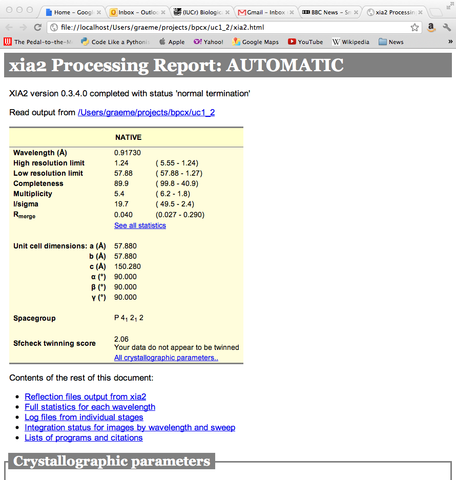
If xia2html has been run there is a nicely formatted html version of this report, which includes graphical representation of some of the log file output from e.g. Scala. Loading up xia2.html will give (hopefully self documenting) results as shown in Figure 5. If you have manually run xia2, immediately running xia2html in the same directory will generate this.
There are a number of program options used on a daily basis in xia2, which are:
| -atom X | tell xia2 to separate anomalous pairs i.e. I(+)≠I(-) in scaling |
| -2d | tell xia2 to use MOSFLM and SCALA |
| -3d | tell xia2 to use XDS and XSCALE |
| -3dii | tell xia2 to use XDS and XSCALE, indexing with peaks found from all images |
| -2da | tell xia2 to use MOSFLM and AIMLESS |
| -3da | tell xia2 to use XDS and XSCALE, merging with AIMLESS |
| -3daii | tell xia2 to use XDS and XSCALE, merging with AIMLESS, indexing with peaks found from all images |
| -xinfo modified.xinfo | use specific input file |
| -image /path/to/an/image.img | process specific scan |
| -spacegroup spacegroup_name | set the spacegroup, e.g. P21 |
| -cell a,b,c,α,β,γ | set the cell constants |
| -small_molecule | process in manner more suited to small molecule data |
Options running Aimless are able to cope with an extremely large number of images - i.e. many thousands, useful when trying to merge data from a number of crystals each with a large number of images, though time consuming!
The subject of resolution limits is one often raised - by default in xia2 they are:
 > 2
> 2
 > 1
> 1However you can override these with -misigma, -isigma.
xia2 depends critically on having CCP4 and CCTBX available. However to get access to the full functionality you will also need XDS and Phenix (which includes Labelit and CCTBX.) Therefore for a “standard” xia2 installation I would recommend:
By and large, if these instruction are followed you should end up with a happy xia2 installation. If you find any problems it’s always worth checking the blog (http://xia2.blogspot.com) or sending an email to xia2.support@gmail.com.
A question often asked is “which options work best” to which the answer is always “it depends!” This is primarily because the outcome of the analysis depends more on the quality of the data than anything else. However I would always try for yourself and get a feel for how the program works for your data - running both -2d and -3d will simply require more computing time / disk space rather than more effort, so it is certainly worthwhile. For small molecule data though -3dii -small_molecule is a good mix. Also -3d often works better for very finely sliced data.
This manual may be cited freely, however it is preferred that references to the use of xia2 be made to Winter, G. Journal of Applied Crystallography (2010) 43, 186-190. Please also remember that the programs that xia2 has used must be correctly cited.
1A.G.W. Leslie, Acta Cryst. (2006) D62, 48-57
2W. Kabsch, Acta Cryst. (2010) D66, 125-132
3P. Evans, Acta Cryst. (2006) D62, 72-82
4CCP4, Acta Cryst. (1994) D50, 760-763
5N.K. Sauter et al. J. Appl. Cryst. (2004) 37, 399-409
6P. Evans, Acta Cryst. (2006) D62, 72-82
7R.W. Grosse-Kunstleve et al. J. Appl. Cryst. (2002) 35, 126-136
8To use -xparallel you will need to fiddle with forkintegrate in the XDS distribution