Latest developments in Diffraction Image Library

Francois Remacle, Graeme Winter,  STFC Daresbury Laboratory Warrington WA4 4AD, United Kingdom

Introduction

This library provides a single way of handling diffraction image that can be originally of various different formats. It has been designed so that you only need to use a single object whatever the format of your image is. All the work of identifying what type of image is done internally.

Alternatively you can come and see me at the BSR conference in manchester where I will be presenting a poster on the Diffraction Image Library.

idiffdisp (CCP4i diffraction image display)

As a first application to use Diffraction Image library, this image viewer will be incorporated in release 6.1 of ccp4. Below is a screenshot of what the main window looks like after opening a single image. The name idiffdisp might change in the future.

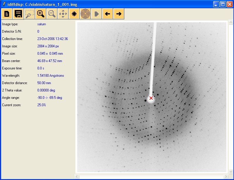
As you can see it is divided in 3 parts: The toolbar, the information panel on the left, originally containing the header information and the zoom level and the image on the right. Let's quickly explain the toolbar.

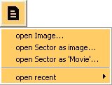	Open menu: Let you open a single image, a maximal image from a sector or make a movie sequence out of a sector. Also give you the possibility to reopen recently opened image/sectors.
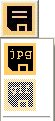
	Save menu: Let you save a single image or a maximal image to jpeg format or save a movie sequence as a gif file. This require image magick convert program to be installed.
	Zoom in and out: from a range of zoom, currently 10%, 25%, 33%, 50%, 66%, 100%, 200%.
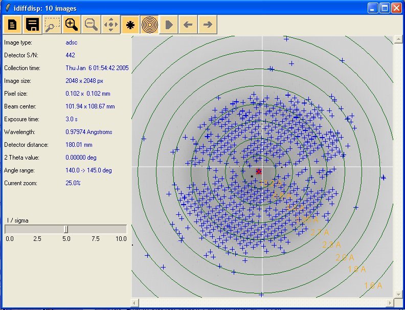
	spots finding: Show/Clear spots found on the image, the original I/sigma value is 2.0 but as soon as this option is on. A slider will appear on the left panel to let you adjust the value as shown with the maximal image screenshot below.
	Resolution circles: Show/clear resolution circles calculated for the image of maximal image.
	Play: Play the movie sequence, only available in movie mode. Note that in movie mode similarly to the I/sigma slider. Two slider appears on the left panel. The first one let you specified the inter frame delay and the second let you slide through your frames. Further to these slider a checkbox appear to let you choose if you want the movie to rollback or not.
	Previous/Next: In image mode, these will open the previous/next image in directory. In movie sequence mode this will display the previous/next frame.

There are a couple of button that are present but not active yet as the function behind them are still being developed. Below you can see an example of a maximal image with spots and resolution circles

Finally, here is an example of a saved movie sequence done with the option save as gif.

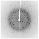
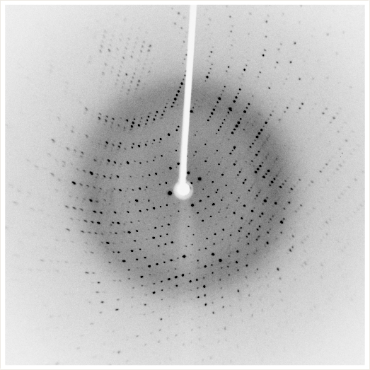
Automask

This is a new function that is still being developed but that already provides very promising results in automatically generating a mask for the backstop area and the arm of the backstop (if present on the image).  Here is a quick description of the way it works.

The first step is to try to determine the backstop area. To do so we shoot rays in 3 different directions 120 degrees apart from each other. We decide to stop as soon as the standard deviation becomes "too big" in comparison with the average pixel count along the rays. With the 3 points obtained we fit a circle passing through them. We repeat the process 10 times changing the initial direction. We then take the average centre coordinates and the largest radius to be the characteristics of our backstop area. We then try to modify it a bit by try to move/grow the circle around to see if there is any direction in which we would lower the standard deviation of the whole disc, and stopping to grow if the standard deviation gets too big.

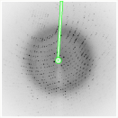
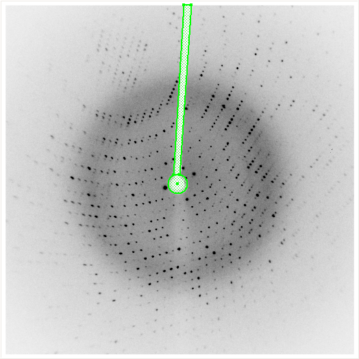
The second step is to determine in which direction the arm of the backstop is situated, and mainly if there is an arm at all. To do so, we shoot 360 degrees rays from centre and as before we stop if the standard deviation of the pixel count gets too big compared to its average value. If by chance we reach the edge of the picture before that than we consider that there is an arm and we use that direction to determine it. If after doing a 360 degree search we did not find a direction where we reached the edge. We try to refine the best result (i.e the direction where we when the farest from the centre) by starting not from the centre of the backstop circle but from its edge. We then restart the search around the best direction so far. If after refining we still did not find any direction we consider there is no arm to the backstop.

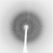
The third step happens when we successfully detected an arm direction. We firstly try to do a simple fitting. To do so, starting from the edge of the backstop circle in the direction found, we shoot two rays parallel to the edge of the picture we touched, one in each direction (i.e left and right or up and down depending on which edge of the picture we stopped). We then shoot another two rays from the edge of the picture. With the four points found we can fit a quad to cover the arm. To see if we consider the quad acceptable we evaluate the average and standard deviation of the pixel count within the quad. 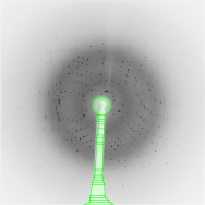If it is not too big we consider we have our solution. If it is too big we consider that the shape of the arm might be tricky and we perform a complex fitting. The complex fitting works the same way as the simple fitting does, but instead of doing the ray shooting at both end we do it 40 times along the direction of the arm. We try to reduce the number of quads by looking at the angles between their edges. If their are flat enough we merge then into one.

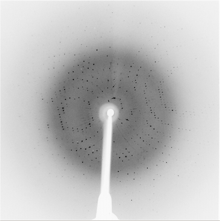
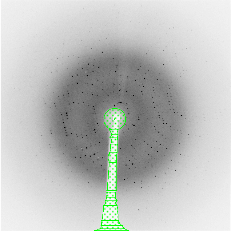
Currently the algorithm is being developed on single image, but in the end it is likely to take the form a command line application that will use from 1 to n images, calculate the minimal image  and perform the mask search on them to avoid interferences when spots are nearby the mask edges. Below are an example of a single fit and a complex fit using single images.

Click on the pictures to enlarge them

Acknowledgments