Newsletter contents...

On the density modification at very low resolution

Abstract

The current techniques for ab initio macromolecular phasing are applicable at very low resolution and need to be followed by some phase extension procedures in order to improve the obtained image. Density modification methods can be used for this image improvement. Since they are usually applied at medium and high resolution (d < approx. 6 Å), a preliminary analysis of the applicability of these methods at very low resolution becomes necessary and is reported here.

I. Introduction

While direct methods for small molecules have become an usual crystallographic tool, the solution of the phase problem for large macromolecules needs extra information like heavy atom derivatives or anomalous dispersion. During recent years some progress in the development of ab initio phasing methods at very low resolution has been reported (see, for example, Lunin, Urzhumtsev and Skovoroda, 1990; Subbiah, 1993; Harris, 1995; Volkman et al., 1995; Lunin et al., 1995, Urzhumtsev & Podjarny, 1995a, Andersson & Hovmöller, 1996; see also the review by Podjarny & Urzhumtsev, 1997). In particular, these methods have obtained the first crystallographic image for the 50S ribosome particle from Thermus thermophilus (Volkman et al., 1995; Urzhumtsev, Vernoslova and Podjarny, 1996). However, the resolution which can be obtained today by these methods is not high enough. A possible way to get a higher resolution image is to develop further the methods like FAM (Lunin et al., 1998; its development and application to the T50S ribosome data allowed an increase in the resolution from 100 Å initially to about 30 Å). Another way is to create or to modify existing methods for image improvement. These methods have been developed to be applied at "usual" resolution (2-5 Å) therefore at very low resolution some basic hypotheses may be not fulfilled. A special analysis should be done in order to show how these methods should be updated, if possible, to be applied at very low resolution data.

One of the basic groups of methods for image improvement is density modification (see, for example, Podjarny, Rees and Urzhumtsev, 1997). The usual iteration procedure of modification of the density distribution function, depending either on the density value in a given point or on the coordinates of this point, can be eventually applied at any resolution. The simplest information which can be used is the flat density in the solvent region (Bricogne, 1974). The following basic questions should be analysed :

1. is such flattening applicable at low resolution (i.e., are structure factors recalculated at the same resolution close enough to the correct values) ?
2. can such procedures extend the phases at low resolution (do phases of structure factors at higher resolution have any structural information) ?
3. can the phase information be improved only by refining the envelope border (flat envelope) or are density values important ?
4. if the procedure is applicable, which are the optimal parameters ?

II. Computational experiment

Test calculations have been carried out using model data calculated from a density modulated envelope for the 50S ribosomal particle (Berkovich-Yellin, Wittmann & Yonath, 1990) arbitrarily placed in the experimentally observed unit cell (space group P43212; a = b = 496Å, c = 196Å) as described before in Lunin et al. (1995). Since no molecular model was used in the procedure, the contribution of the disordered solvent (Urzhumtsev & Podjarny, 1995b) was not taken into consideration. No experimental error was introduced.

The following procedure has been applied :

1. calculate a density distribution at a given resolution (60, 40 or 30 Å);
2. define a molecular envelope as a set of unit cell points with the density value above a given threshold; the threshold was defined to leave a given percentage of the unit cell volume above this level;
3. flatten the density distribution below the threshold keeping the density above the threshold ("soft modification"); alternatively, at the test for using flat envelopes, the density above the threshold was also flattened ("hard modification");
4. calculate structure factors form the modified density distribution;
5. compare calculated structure factors with the exact values

We considered that "good" structure factors at the starting resolution indicate the applicability of such flat solvent hypothesis (or flat envelope hypothesis), and that "good" phases at higher resolution indicate the possibility to use such procedure for image improvement. The limit of "goodness of added phases" was taken as 60 degrees (mean cosine value is 0.5) following Lunin & Woolfson (1993). Note that no iterations were done, all numbers are shown for structure factors obtained after a single density modification.

III. Table explanation

The procedure was applied for the maps of the resolution of 60, 40, 30 Å. Tables 1-3 give the results of the comparison of structure factors. Different columns correspond to different cut-off level values varied from 10 to 90% (percentage of the volume above the threshold value).

The amplitude correlation was calculated for Fobs (simulated data set) and Fcalc (after density modification) around their mean values.

The weighted phase correlation was calculated as the mean value of cos() weighted by Fobs**2, which corresponds to the closeness of the maps calculated with Fobs and with exact or calculated phases.

Cells are coloured accordingly to the criteria value; for the phase difference the limit value is 60 degrees. The shell of reciprocal space corresponding to the resolution slightly higher than the starting one is analysed in more detail and is given at the bottom of every table.

Table 1.1. Starting density at 60 Å; "hard" modification

Table 1.1c. Mean , in degrees

Table 1.2. Starting density at 60 Å; "soft" modification

Table 1.2c. Mean , in degrees

Table 2.1. Starting density at 40 Å; "hard" modification

Table 2.1c. Mean , in degrees

Table 2.2. Starting density at 40 Å; "soft" modification

Table 2.2c. Mean , in degrees

Table 3.1. Starting density at 30 Å; "soft" modification

Table 3.1c. Mean , in degrees

IV. Results and discussion

The following observations can be made :

1. The structure factors, calculated at the same resolution as the starting synthesis, are close enough to the correct values, which means that the hypothesis on the flat solvent can be used at such resolution.
2. For the structure factors calculated in higher resolution shells, the calculated amplitudes are not so good. However, in many cases the phases in the closest resolution shell have sufficiently high quality to be used to improve the starting image.
3. The results obtained by the "soft" modification, i.e. when the highest density distribution values are not changed (keeping the density "inside the envelope") are much less sensitive to the threshold level. Note that a similar observation was found for the molecular replacement searches with an envelope (Urzhumtsev & Podjarny, 1995a).
4. The hard modification is significantly less useful at 40 Å than at 60 Å. It means that at such (and higher) resolution the phase extension cannot be achieved by a simple refinement of the envelope border and needs the knowledge of density distribution values.
5. It is interesting to note that in several cases (for example, Tables 2.2) a "wave effect" can be observed : when starting from the 40Å -resolution map, the amplitudes and the phases in the resolution shell 35-37 Å are better than those in the resolution shell 37-40 Å. However, it could be a purely statistical effect.
6. The density modification became more efficient when increasing the resolution of the starting synthesis.
7. Optimal cut-off level does not necessarily correspond to the correct molecular volume (in this case it was about 35 percent).

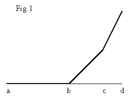As was discussed by Lunin (1988), the basic idea which is behind most of density modification procedures and which defines the form of the density modification function is the closeness of the electron density histograms. In our case, the corresponding histograms have been calculated at different resolution from 20 to 90 Å. We have no possibility to discuss here the details of this analysis and can only mention that the density modification function corresponding to the optimal density modification from 90 to 20 Å resolution maps can be nicely approximated by a function schematically presented in Figure 1 : at the interval (a,b) it corresponds to the solvent flattening, at the interval (b,c) it "keeps" the density values and the interval (c,d) the function needs to sharpen the highest density values. In general, this function supports the idea of "soft" modification. The application of histogram-fitted density modification will be discussed elsewhere.

References

Newsletter contents ...