------------ CCP4 Newsletter - June 1996 ------------
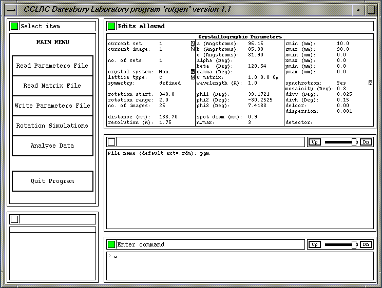
Figure 1. Main Screen of ROTGEN
The current program incorporates functions from the CCP4 (Collaborative Computational Project, Number 4, (1994)) and/or the MOSFLM suite (Wonacott, Dockerill & Brick (1980), Lesli;e (1992)) programs OSCGEN, UNIQUE and COMPLETE (the function of the latter now incorporated in MTZDUMP). The general treatment of the goniometry is derived from that used in the MADNES program (Messerschmidt & Pflugrath, 1987). The program makes also use of the XDL_VIEW toolkit (Campbell, 1995), library routines from the Daresbury Laboratory Laue Software Suite (Helliwell et al., 1989) and the CCP4 libraries.
The program is a first stage in an on-going development; the main aim in the next stages of development is to provide strategy information for efficient data collection using the rotation method. If successful procedures are developed, it may well be desirable to integrate the use of the program, perhaps in a re-packaged form, with the PXGEN interface used on PX stations 9.5 and 7.2 at the Daresbury SRS (Kinder, McSweeney & Duke (1996). It is intended however that a stand alone version will also be retained.
The most immediate next steps are to allow the input of previously collected data (from an MTZ file) to be read into the program and included in the data coverage analyses and to provide quicker though slightly approximated analyses.
The parameters in the main parameter table are assigned default values when the program is started. Individual parameters may be reset by editing the values directly in the parameter table. A new set of parameters may be read in from a keyworded parameters file using the 'Read Parameters File' option.
When the required parameters have been set up, they may be saved in a keyworded parameters file for future use using the 'Write Parameters File' option.
The 'Read Matrix File' option may be used to reset the parameters which define the crystal orientation using matrices produced following auto-indexing by programs such as REFIX or DENZO.
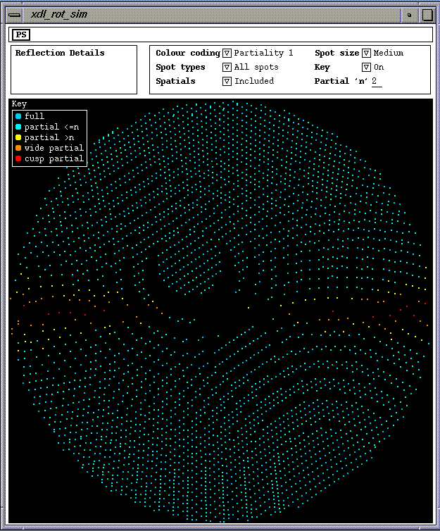
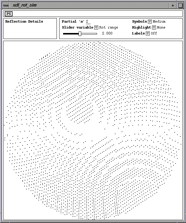
Two basic types of simulations are available, 'colour' simulations and 'interactive' simulations. In each case a window is created with a display area for the simulation, an area to list details of a selected reflection, a control panel and an area used for requesting hard copy (Postscript) output of the simulation. 'Colour' simulations show the show the rotation patterns with the spots colour coded in a number of different ways. 'Interactive' simulations are in black and white and have a slider which allow the user to investigate the effects of changing various parameters such as the oscillation range and mosaicity; spot labelling is also available.
This option enables the prediction of the reflections which would be recorded for the defined crystal sets and to analyse the data coverage in terms of the unique data for the space group, cell and resolution. The analysis may be done for either the current crystal set or for all crystal sets within the data set. The results may be presented in the form or histograms describing the data coverage or in terms of a pictorial representation of the reciprocal lattice sections. The analysis data equivalent to that displayed in the histograms is also written to the log file. The analyses automatically written to the log file exclude any spatially overlapped reflections.
The parameters include specifications for one or more crystal orientations and sets of images. Some parameters refer to the dataset as a whole and some may have separate values for each of the crystal sets.
A general Keyword Data Module (KDM) set of functions is used by ROTEGEN to define and handle its keyworded data set. It uses many the same concepts as the Laue Data Module (Campbell, Clifton, Harding & Hao, 1995) but the KDM routines are general whereas the LDM routines were written for a specific set of parameters. The KDM routines enable parameters of various types to be defined e.g. integer, real or character. Additional sets of routines are used to handle the input and output of KDM data and also symmetry data (KWD and KSM routines).
For most parameters a keyword is followed by a single value. The keywords are case insensitive and need not be given in full though a certain minimum number of characters must be given in each case. For a set based parameter the keyword may have a set number appended in square brackets e.g. ROTSTART[2] 50.0; if the set number is omitted, it is assumed that the value following the keyword refers to all sets e.g. RESOLUTION 2.0.
KDM Routines enable the monitoring of changes to KDM parameter values during the execution of a program. KWD/KDM based data files may contain indirect references to data in another file by giving a file name reference of the form '@filename'. These indirect files may currently be nested to a level of up to 20.
When a MOSFLM suite matrix file is input, the following parameters are updated:
For a DENZO file input, the following parameters are updated:
In contrast to the MOSFLM case, the missetting angles and cell need to be derived from the matrix read in as the required values are not stored in the file. The program derives the missetting angles on the basis of the current value of the U-matrix and this remains unchanged again in contrast with the MOSFLM case.
Figure 2. Example of a Colour Rotation Simulation
Control Panel Options
The colour coding depends on the option selected via the Colour coding choice menu on the control panel. The display is qualified by the settings of other control panel items. The options available are:
  blue:    fulls
  yellow:  partials (up to maximum used in the prediction)
  red:     cusp partials
 blue:    fulls
 cyan:    partial <=n as set in the Partial 'n' panel item
 yellow:  partial >n and up to the maximum used in the
          prediction
 orange:  wide partial (greater than the maximum partiality
          used in the prediction)
 red:     cusp partial
 blue:    fulls
 cyan:    partial =2
 green:   partial =3
 yellow:  partial >3 and up to the maximum used in the
          prediction
 orange:  wide partial (greater than the maximum partiality
          used in the prediction)
 red:     cusp partial
 blue:    not overlapped
 yellow:  spatially overlapped spot
The 'Spot types' choice menu on the control panel allows the user to choose one of the following three options:
The display of spatially overlapped spots may be controlled via the 'Spatials' choice menu on the control panel. There are three options:
The user may select one of three spot sizes, small medium or large for the display via the 'Spot size' choice menu on the control panel.
The display, of a key at the top left of the display area showing the colour coding, may be turned on or off via the 'Key' choice menu on the control panel.
The partial 'n' value, used in deciding which category a partial spot is to be included in for the Partiality 1 colour coding option a nodal can be reset via the Partial 'n' value item on the control panel. The value must be in the range of 2 to the maximum value used in the prediction.
Listing Spot Details
When the mouse Button1 is pressed with the cursor on a spot position, details of that spot will be listed in the spot details area. The following information is listed:
The selected spot is marked by a surrounding white circle on the display area. The selection may be removed by clicking Button2 or Button3 of the mouse (or Button1 when the cursor is within the display area but not pointing to a spot). When Button1 is pressed, the nearest spot to the cursor is selected provided that the distance squared (pixels) to the spot is no more than 18.
Hard Copy
To get a hard copy plot in the form of a Postcript file, select the panel button marked PS in the hard copy request area at the top of the view object. A question and answer sequence is then followed using a panel i/o item to the right of the PS button. Invalid replies will give pop-up error notices. The hard copy output may be abandoned by pressing the Escape key when a prompt is displayed.
Figure 3. Example of an Interactive Rotation Simulation
Control Panel Options
A 'Slider variable' panel choice item determines which of the available variable parameters can currently be adjusted via the slider. The parameters which may be varied under slider control are:
The use of the slider was originally designed for use on colour displays which have 'writeable colour maps'. In fact 50 colours are used on the display with the spots being 'colour coded' by the value of the current variable parameter. The 50 colours are then set to white or black depending on the position of the currently selected slider. If the slider is moved then the display is altered merely by changing the colours in the colour map thus giving a rapid change of pattern as the slider is moved. On displays which do not have writeable colour maps and on monochrome displays, the use of the sliders is less effective as the pattern needs to be redrawn each time a slider is moved.
The current value for the parameter being varied is displayed to the right of the slider. The overall range is defined by the calling program.
The 'Highlight' choice menu on the control panel may be used to enable various classes of spots to be highlighted. The options available are as follows:
Note: When spots are highlighted and the soft limit sliders are used, the plot will be redrawn each time a slider is moved. The sliders are best used when no spots are highlighted.
The user may select one of three spot sizes, small medium or large for the display via the 'Symbols' choice menu on the control panel.
The partiality value defining the boundary between the two main classes of partials may be set via the Partial 'n' value item on the control panel. The value must be in the range of 2 to the maximum value used in the prediction.
The 'Labels' choice menu allows a number options for labelling. These are:
If there are labels already displayed when a new labels option is selected, the existing labels will be redrawn as needed.
Note: When labels are displayed the plot may be redrawn if the slider is moved because a spot has disappeared or reappeared. The sliders are best used when no labels are displayed.
Listing Spot Details
When the mouse Button1 is pressed with the cursor on a spot position, details of that spot will be listed in the spot details area. The following information is listed:
The selected spot is marked by a surrounding red circle on the display area (black on a monochrome display). The selection may be removed by clicking Button1 when the cursor is within the display area but not pointing to a spot. When Button1 is pressed, the nearest spot to the cursor is selected provided that the distance squared (pixels) to the spot is no more than 18.
The spot details are also listed when a spot is labelled.
Labelling Spots
Providing that one of the labelling options has been selected via the 'Labels' choice menu, spots may be labelled on the plot. The labels are positioned under user control.
Hard Copy
To get a hard copy plot in the form of a Postcript file, select the panel button marked PS in the hard copy request area at the top of the view object. A question and answer sequence is then followed using a panel i/o item to the right of the PS button.
When the analysis is initiated, the program first calculates a list of the unique reflections for the spacegroup and cell based on the resolution of the first crystal set defined. The program outputs a message for each crystal set for which predictions are being done. If there is more than one image in the set, then, a progress bar will be displayed to indicate the progess of the predictions throughout the images of the set. A cancel button is also displayed in case the user wishes to abandon the analysis before it has been completed.
The results may be presented in the form or histograms describing the data coverage or in terms of a pictorial representation of the reciprocal lattice sections.
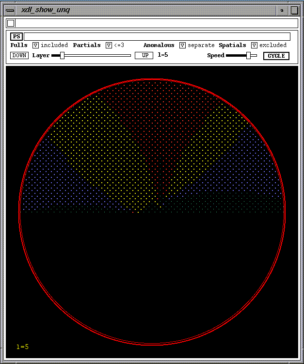
Figure 4. Example of 'Show Unique Coverage' View-object
The points on the unique part of the reciprocal lattice are marked by small greenish dots for those spots which have not been predicted/measured. Where anomalous data are merged, all predicted/measured reflections are represented by yellow dots. Where the anomalous data are to be separated the following colour coding is used.
       yellow:    Both an I+ and an I- reflection are present.
       red:       Only the I+ reflection is present.
       blue:      Only the I- reflection is present.
       white :    Unknown sign (i.e. both I+ and I- are not present
                  though I+ or I- may be present in addition to
                  measurements flagged as being of unknown sign.
All the plots currently available are plots against resolution. The resolution range, from infinity to the resolution limit defined for the first crystal set, is divided into ten equal bins of 4.sin**2(theta)/lambda**2. The three plots are as follows:
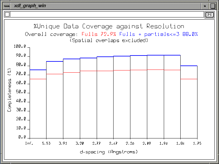
This plot shows the percentage of coverage of the unique data within each resolution bin. Where partials are included two lines are drawn, a blue one indicating the coverage for the full reflections plus the included partials and a red one indicating the coverage for the full reflections only. The overall percentage coverage for each of these cases is given at the top of the plot. Where no partials are included a blue line indicates the coverage by the fulls data and the overall coverage by the fulls data is given at the top of the plot.
Figure 5. Example of a Unique Data Coverage Graph
This plot shows the average reflection measurement multiplicity within each resolution bin. Where partials are included in the analysis two lines are drawn, a blue one indicating the multiplicity for the full reflections plus the included partials and a red one indicating the coverage for the full reflections only. The overall average multiplicity for each of these cases is given at the top of the plot. Where no partials are included a blue line indicates the average multiplicity of the fulls data and the overall average multiplicity of the fulls data is given at the top of the plot.
The analyses automatically written to the log file exclude any spatially overlapped reflections. If the user also wishes to have analyses with the spatially overlapped reflections included, then these must be specifically requested.
When a new parameters file is read in, the values of the keyworded parameters are written to the log file.
When a data analysis has been carried out, then any keyworded parameter values, which have been changed since reading in a new parameters file or since the previous analysis, are written to the log file. Three analyses tables are output in a form which may be accessed by the CCP4 'xloggraph' program if desired. These are for unique data coverage, acentric pairs coverage and reflection multiplicity. All are shown as functions of resolution in 10 resolution bins. These analyses exclude spatially overlapped reflections.
Analogous analyses including spatially overlapped reflections will only be written to the log file if this was specifically requested when examining the analysis results in ROTGEN.
When the program is terminated, the current values of the keyworded parameters are written to the log file.
The use of the 'Rotation Simulations' option does not result in any additional log file output.
General, Crystal System and AlignmentTitle TITLE A title for the dataset.
No. crystal sets NUMSETS Number of crystal sets defined within this dataset.
Crystal system SYSTEM The crystal system Tri, Mon, Ort, Tet, Hex, Rho or Cub.
Lattice type LATTICE Lattice type P, A, B, C, I, F or R.
Crystal symmetry SYMMETRY The space group symmetry followed by the space group number, space group name or symmetry operators (or 'clear' to clear the current symmetry).
Cell, Resolution, Wavelength and Orientation Parameters
Cell A[], B[], C[], ALPHA[], BETA[], GAMMA[]
The cell parameters in Angstroms and degrees.
Resolution RESOLUTION[] The resolution limit in Angstroms.
Wavelength WAVELENGTH[] The wavelength in Angstroms.
U-matrix UMATRIX[] The basic 'U' setting matrix (9 values).
Missetting angles PHI1[], PHI[2], PHI3[]
The misseting angles in degrees.
The Rotation Ranges, Mosaicity and Spot Sizes
Rotation start ROTSTART[] Rotation start angle in degrees.
Oscillation range OSCRANGE[] Oscillation range in degrees (+ve).
No. of images NUMIMG[] No. of images to collect.
Partials limit NWMAX[] Only consider partials occurring on up to this number of images.
Mosaicity MOSAICITY[] The mosaic spread in degrees.
Spot size SPOT_SIZE[] The spot diameter in mm.
Detector Parameters
Distance DISTANCE[] The crystal to detector distance in mm.
Rmin RMIN[] Minimum radius on detector in mm.
Rmax RMAX[] Maximum radius on detector in mm.
Limits XMIN[], XMAX[], YMIN[], YMAX[]
Detector limits on 'x' and 'y' from pattern centre (mm.).
Orientation DET_ROTATIONS[] Directions of three orthogonal detector rotation axes.
Axes DET_AXES[] Detector axis vectors
Horizontal axis IAX_H[] Horizontal axis number 1-3.
vertical axis IAX_V[] Vertical axis number 1-3.
Beam vector BEAM_VECTOR[] Beam vector.
Scan axis SCAN_AXIS[] Rotation axis vector.
Other Source Parameters
Synchrotron SYNCHROTRON[] Synchrotron - yes or no.
Dispersion DISPERSION[] The dispersion delta(lambda)/lambda.
Vertical divrg. DIVV[] Vertical divergence in degrees.
Horizontal divrg. DIVH[] Horizontal divergence in degrees.
Corr. dispersion DELCOR[] Correlated dispersion.
Campbell, J.W. "XDL_VIEW, an X-windows-based toolkit for crystallographic and other applications" J. Appl. Cryst. (1995) 28 236-242
Campbell, J.W., Clifton, I.J., Harding, M.M. and Hao, Q., "The Laue Data Module (LDM) - a software development for Laue X-ray diffraction data processing" J. Appl. Cryst. (1995) 28 635-640
Collaborative Computational Project, Number 4 "The CCP4 Suite: Programs for Protein Crystallography" Acta Cryst. (1994) D50 760-763
Helliwell J.R., Habash J., Cruickshank D.W.J., Harding M.M., Greenhough T.J., Campbell J.W., Clifton I.J., Elder M., Machin P.A., Papiz M.Z. and Zurek S. "The Recording and Analysis of Synchrotron X-radiation Laue Diffraction Photographs" J. Appl. Cryst. (1989) 22 483-497
Kinder S.H., McSweeney S.M. and Duke E.M.H. "PXGEN: A general purpose graphical user interface for protein crystallography experimental control and data acquisition" J. Appl. Cryst. (1996) submitted for publication.
Leslie A.G.W. In CCP4 and ESF-EACBM Newsletter on Protein Crystallography (1992) No. 26, DRAL Daresbury Laboratory, Warrington, WA4 4AD, England
Messerschmidt A. and Pflugrath J.W. "Crystal orientation and X-ray pattern prediction routines for area detector diffractometer systems in macromolecular crystallography" J. Appl. Cryst. (1987) 20 306-315
Wonacott A.J., Dockerill S. and Brick P. "MOSFLM program" (1980) Unpublished Notes.