Exploring Metric Symmetry
P.H. Zwart, R.W. Grosse-Kunstleve & P.D. Adams
Lawrence Berkeley National Laboratory, 1 Cyclotron Road, BLDG 64R0121, Berkeley, California 94720-8118, USA. Email: PHZwart@lbl.gov; www: http://cci.lbl.gov
1. Introduction
Relatively minor perturbations to a crystal structure can in some cases result in apparently large changes in symmetry. Changes in space group or even lattice can be induced by heavy metal or halide soaking (Dauter et al, 2001), flash freezing (Skrzypczak-Jankun et al, 1996), and Se-Met substitution (Poulsen et al, 2001). Relations between various space groups and lattices can provide insight in the underlying structural causes for the symmetry or lattice transformations. Furthermore, these relations can be useful in understanding twinning and how to efficiently solve two different but related crystal structures. Although (pseudo) symmetric properties of a certain combination of unit cell parameters and a space group are immediately obvious (such as a pseudo four-fold axis if a is approximately equal to b in an orthorhombic space group), other relations (e.g. Lehtio, et al, 2005) that are less obvious might be crucial to the understanding and detection of certain idiosyncrasies of experimental data.
We have developed a set of tools that allows straightforward exploration of possible metric symmetry relations given unit cell parameters and a space group. The new iotbx.explore_metric_symmetry command produces an overview of the various relations between several possible point groups for a given lattice. Methods for finding relations between a pair of unit cells are also available. The tools described in this newsletter are part of the CCTBX libraries, which are included in the latest (versions July 2006 and up) PHENIX and CCI Apps distributions.
2. Methods
2.1. Determination of the lattice symmetry
The determination of the lattice symmetry is based on ideas by Le Page (1982) and Lebedev et al. (2006). Given a reduced cell (e.g. Grosse-Kunstleve et al. 2004a), it is sufficient to search for two-fold axes to determine the full symmetry. Subjecting the two-folds to group multiplication produces the higher-order symmetry elements, if present.
Le Page (1982) searches for the two-folds by computing angles between certain vectors in direct space and reciprocal space. This search is relatively expensive. Recently Lebedev et al. (2006) introduced the idea of simply enumerating all 3x3 matrices with elements {-1,0,1} and determinant one. As an additional requirement group multiplication based on each matrix individually has to produce matrices exclusively with elements {-1,0,1}. There are only 480 matrices that conform to all requirements. Lebedev et al. (2006) argue that this set covers all possible symmetry operations for reduced cells. We were able to confirm this intuitive argument empirically via simple brute-force tests.
Only 81 of the 480 selected matrices correspond to two-folds. These are easily detected by establishing which of the matrices produce the identity matrix when multiplied with themselves (and are not the identity matrix to start out with). To replace the expensive search for two-folds in the original Le Page (1982) algorithm, the 81 two-fold matrices are tabulated along with the axis directions in direct space and reciprocal space. The axis direction in direct space is determined as described by Grosse-Kunstleve (1999). The axis direction in reciprocal space is determined with the same algorithm, but using the transpose of the matrix. The complete implementation of the algorithm for generating the table (essentially just six lines of Python code) can be found in the file cctbx_sources/cctbx/cctbx/examples/reduced_cell_two_folds.py in the cctbx distributions.
The search for two-folds computes the Le Page
(1982)  for each of the 81 tabulated pairs of axis directions. The corresponding
symmetry matrix for each pair is immediately available from the table. In
contrast, the original Le Page algorithm requires the evaluation of 2391 pairs
of axis directions, and the computation of the symmetry matrices involves
expensive trigonometric functions (sin, cos) and change-of-basis calculations.
for each of the 81 tabulated pairs of axis directions. The corresponding
symmetry matrix for each pair is immediately available from the table. In
contrast, the original Le Page algorithm requires the evaluation of 2391 pairs
of axis directions, and the computation of the symmetry matrices involves
expensive trigonometric functions (sin, cos) and change-of-basis calculations.
The matrices with a Le Page
smaller than a given threshold are sorted, smallest
first. Successive group multiplication as described in Grosse-Kunstleve et al.
(2004b) and Sauter et al. (2006) yields the final highest lattice
symmetry. The complete search algorithm is implemented in the file
cctbx_sources/cctbx/sgtbx/lattice_symmetry.cpp.
Since the algorithm determines the lattice symmetry in a primitive setting (the reduced cell), the resulting symmetry matrices do not in general correspond to one of the usual space group settings for which a Hermann-Mauguin symbol is available. However, all lattice symmetries can be exactly characterized with Hall symbols. In contrast to Hermann-Mauguin symbols, Hall symbols uniquely define the orientation of the symmetry elements with respect to the cell axes. This property is vital for understanding relations between different point groups.
2.2. Construction of a point group graph
In order to be able to systematically explore various possible point groups for a given set of unit cell parameters, a graph is constructed that encodes group-subgroup relations between various point groups. A graph is constructed in the following manner:
-
The lattice symmetry of the Niggli cell is deduced, as described above.
-
Starting from the base point group (P1 or the point group corresponding to a user specified space group), each symmetry elements from the point group of the lattice not present in the base point group is combined with the base point group to generate a supergroup.
-
The former procedure is carried out for the newly generated point groups. The procedure is iterated until no new point groups are generated. The relations between the constructed point groups are described in a graph.
The resulting point group graph can be used to visualize relations between various symmetries or could be used to systematically assess the validity of a number of intensity symmetry hypotheses. It is important to note that the set of relations generated in this manner only describe the change in point group upon addition or removal of rotational symmetry, but does not cover changes due to addition or removal of translational symmetry.
2.3 Generation of compatible space groups
Only a limited set of space groups are compatible with a given point group of the lattice. This set of space groups compatible with a certain point group is for instance used in molecular replacement when the space group is not known.
To further limit the set of set of compatible space groups, it is assumed that systematic absences dictated by the user supplied space group have to be retained. However, this set of systematic absences is not assumed to be complete.
The list of possible space groups derived for each point group is constructed while ensuring that systematic absent Miller indices in the user supplied space group will also be absent. Non-absent reflections in the user supplied space group are not required to be non-absent in the new space group.
A simple example illustrates the described rules in the selection of possible space groups. If the symmetry of the lattice is P 2 2 2 and the user-supplied space group is P 21 21 2, the possible space groups are P 21 21 2 and P 21 21 21. The space group P 2 2 2, 3 settings of P 2 2 21 and 2 settings of the space group P 21 21 2 all violate the systematic absences dictated by the user-supplied space group.
2.4. Sub-lattice generation
Although the above methods allow the user to inspect the effect of removal or addition of rotational symmetry in the lattice, space group transitions often involve a change in the reduced cell volume as well.
Generation of all sub-lattices that result in a
certain volume change, can be obtained by generating all matrices  with integer indices that have a determinant equal to the desired change in
volume of the reduced cell. The resulting sublattice is than obtained from the
original lattice via the relation:
with integer indices that have a determinant equal to the desired change in
volume of the reduced cell. The resulting sublattice is than obtained from the
original lattice via the relation:

Generating all matrices with a specified determinant in a naive manner by looping over all matrix elements within in fixed range (say from -5 to 5) is however impractical (approximately 2.4 10^9 iterations). A more practical solution lies in the fact (Billet & Rolley Le-Coz, 1980; Rutherford, 2006) that it is sufficient to only generate matrices in the Hermite normal form:
The elements of
are all integers. The elements  ,
,
 and
and  are all larger than zero. The restrictions on the values of
  ,
,
 and
and  depend on the diagonal element of the row in which the elements occur :
![$ d,e \in \left[ -(a+1)/2, -(a+1)/2 + 1, \cdots, (a+1)/2 \right] \, a \,\,\mathrm{odd} $](explore_symmetry_files/latex2png_c0ab6e9a0fe5e8022e1fa647d27e3713c5f00c011.png)
![$ d,e \in \left[ -(a/2), -(a/2)+1, ..., (a/2) \right] \, a \,\,\mathrm{even} $](explore_symmetry_files/latex2png_0437115dd11dc1d68d75a9d5c381fa60edd63c541.png)
Similar restrictions for
apply.
Because the determinant (and thus the resulting
volume change) of the matrix is equal to  ,
all matrices with a determinant
,
all matrices with a determinant  can be constructed by generating all triplets
  for which
  holds. Generation of triples is done using an algorithm known as
trial division.
holds. Generation of triples is done using an algorithm known as
trial division.
After generating the new lattice as described above, the new unit cell parameters can be compared to a target unit cell. The new unit cell is reduced to a Niggli cell. The new Niggli cell cannot be compared directly to the target Niggli cell, because small differences in unit cell parameters, can result in large differences in reduced cell parameters (Andrews et al., 1980). Therefore, all unimodular transforms with matrix elements in the range from -1 to 1 are generated. After using these matrices to transform the new Niggli cell, it considered similar to the target Niggli cell if user-defined tolerances on length and angular deviations are fulfilled. An example of this procedure is shown in section 3.2, where two unit cells are compared. The Niggli cell with smallest volume will be used as a building block (denoted Lego cell in the output) to try and construct a unit cell similar to the Niggli cell with the larger volume (denoted as Target cell in the output).
3. Examples
3.1. Incorrectly processed Insulin
An insulin dataset (kindly provided by C.B. Trame, Berkeley Center for Structural Biology) was purposely incorrectly indexed and scaled.
As a test, the data was indexed, integrated and scaled in P1. The resulting cell is equal to:
68.4 68.4 68.3 109.5 109.4 109.5
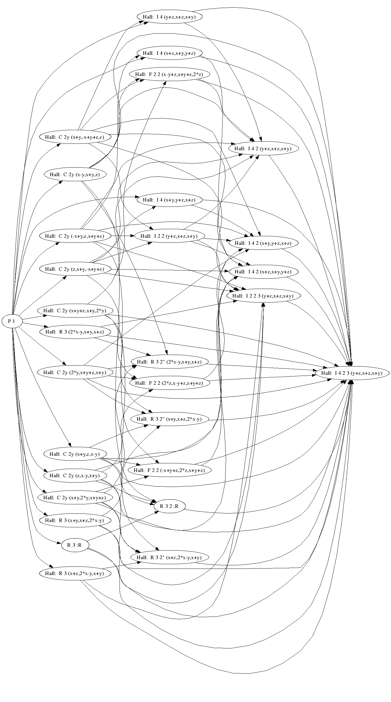
As the symmetry of the lattice is cubic (Hall: I 4 2 3 (y+z,x+z,x+y)), the resulting point group graph contains all point groups between cubic and anorthic (P1) symmetry.
The point group graph generating algorithm is used in Xtriage (Zwart et al, 2005) in order to determine missing rotational symmetry. A scoring function based on R-values (similar to those used by Labelit (Sauter et al., 2006) ) is available to help guide the user to the most likely point group:
------------------------------------------------------------------------------------------------------
| Point group                     | mean R_used | max R_used | mean R_unused | min R_unused | choice |
------------------------------------------------------------------------------------------------------
| Hall:  I 4 (y+z,x+z,x+y)        | 0.309       | 0.436      | 0.280         | 0.042        |        |
| P 1                             | None        | None       | 0.291         | 0.042        |        |
| Hall:  C 2y (2*y,x+y+z,x+y)     | 0.432       | 0.432      | 0.260         | 0.042        |        |
| Hall:  C 2y (x+y,z,x-y)         | 0.436       | 0.436      | 0.295         | 0.042        |        |
| Hall:  C 2y (x+y,-x+y+z,z)      | 0.044       | 0.044      | 0.306         | 0.042        |        |
| Hall:  R 3 (2*x-y,x+y,x+z)      | 0.043       | 0.043      | 0.271         | 0.042        |        |
| R 3 2 :R                        | 0.435       | 0.436      | 0.433         | 0.432        |        |
| Hall:  C 2y (z,x-y,x+y)         | 0.435       | 0.435      | 0.259         | 0.042        |        |
| Hall:  R 3 (x+y,x+z,2*x-y)      | 0.044       | 0.044      | 0.270         | 0.042        |        |
| Hall:  R 3 (x+z,2*x-y,x+y)      | 0.042       | 0.042      | 0.269         | 0.042        |        |
| Hall:  I 4 2 (y+z,x+z,x+y)      | 0.340       | 0.436      | 0.240         | 0.042        |        |
| Hall:  F 2 2 (-x+y+z,2*z,x+y+z) | 0.435       | 0.436      | 0.360         | 0.044        |        |
| Hall:  I 4 (x+z,x+y,y+z)        | 0.307       | 0.435      | 0.280         | 0.042        |        |
| Hall:  R 3 2" (2*x-y,x+y,x+z)   | 0.176       | 0.434      | 0.434         | 0.433        |        |
| Hall:  I 4 2 (x+z,x+y,y+z)      | 0.339       | 0.435      | 0.434         | 0.433        |        |
| Hall:  I 4 2 3 (y+z,x+z,x+y)    | 0.291       | 0.436      | None          | None         |        |
| Hall:  F 2 2 (2*z,x-y+z,x+y+z)  | 0.433       | 0.435      | 0.359         | 0.044        |        |
| Hall:  C 2y (x+y,2*y,x+y+z)     | 0.434       | 0.434      | 0.296         | 0.042        |        |
| Hall:  C 2y (z,x+y,-x+y+z)      | 0.034       | 0.034      | 0.281         | 0.042        |        |
| Hall:  R 3 2" (x+y,x+z,2*x-y)   | 0.434       | 0.436      | 0.176         | 0.042        |        |
| Hall:  I 2 2 3 (y+z,x+z,x+y)    | 0.043       | 0.044      | 0.433         | 0.433        | <---   |
| Hall:  C 2y (x-y,x+y,z)         | 0.435       | 0.435      | 0.224         | 0.034        |        |
| Hall:  F 2 2 (x-y+z,x+y+z,2*z)  | 0.242       | 0.433      | 0.205         | 0.042        |        |
| Hall:  I 4 (x+y,y+z,x+z)        | 0.304       | 0.435      | 0.280         | 0.042        |        |
| Hall:  R 3 2" (x+z,2*x-y,x+y)   | 0.434       | 0.435      | 0.175         | 0.042        |        |
| Hall:  C 2y (-x+y,z,x+y+z)      | 0.042       | 0.042      | 0.281         | 0.042        |        |
| Hall:  I 4 2 (x+y,y+z,x+z)      | 0.244       | 0.435      | 0.434         | 0.433        |        |
| R 3 :R                          | 0.042       | 0.042      | 0.269         | 0.042        |        |
| Hall:  I 2 2 (y+z,x+z,x+y)      | 0.043       | 0.044      | 0.305         | 0.042        |        |
| Hall:  C 2y (x+y+z,x+y,2*y)     | 0.433       | 0.433      | 0.188         | 0.034        |        |
------------------------------------------------------------------------------------------------------


R_used: mean and maximum R value for symmetry operators *used* in this point
        group
R_unused: mean and minimum R value for symmetry operators *not used* in this
          point group
The likely point group of the data is:  Hall:  I 2 2 3 (y+z,x+z,x+y)

Possible space groups in this point groups are:
  Unit cell: (78.9732, 78.9732, 78.9732, 90, 90, 90)
  Space group: I 2 3 (No. 197)

  Unit cell: (78.9732, 78.9732, 78.9732, 90, 90, 90)
  Space group: I 21 3 (No. 199)
3.2. Unit cell comparison
The presence of pseudo symmetric properties of a lattice associated with a set of unit cell parameters, is often discovered at the stage of indexing and scaling the data. If however a derivative or crystal from slightly different crystallization conditions is available, the presence of a relation to the native or other crystal form is often not immediately clear. Using the sublattice tools discussed in section 2.4, relations between two unit cells can easily be determined.
For example, Poulsen et al. (2001) observed crystal of the native protein and two Se-Met derivatives with the following cell parameters and space groups:
Native :  P 21 21 21    61.8   97.7  148.9  90  90  90
SeMet1 :  P 1 21 1     115.5  149.0  115.6  90 115  90 (pseudo hexagonal)
SeMet2 :  C 2 2 21     123.6  195.4  148.9  90  90  90
Comparing Native and SeMet1
Using the command
iotbx.explore_metric_symmetry --unit_cell="61.8 97.7 148.9 90 90 90"
   --space_group=P212121 --other_unit_cell="115.5 149.0 115.6 90 115 90"
   --other_space_group=P21 --no_point_group_graph
The following output is produced:
--------------------
Unit cell comparison
--------------------

The unit cells will be compared. The smallest Niggli cell,
will be used as a (semi-flexible) lego-block to see if it
can construct the larger Niggli cell.

Crystal symmetries in supplied setting
--------------------------------------
Target crystal symmetry:
    Unit cell: (115.5, 149, 115.6, 90, 115, 90)
    Space group: P 1 21 1 (No. 4)
Building block crystal symmetry:
    Unit cell: (61.8, 97.7, 148.9, 90, 90, 90)
    Space group: P 21 21 21 (No. 19)

Crystal symmetries in Niggli setting
------------------------------------
Target crystal symmetry:
    Unit cell: (115.5, 115.6, 149, 90, 90, 115)
    Space group: P 1 1 21 (No. 4)
Building block (lego cell) crystal symmetry:
    Unit cell: (61.8, 97.7, 148.9, 90, 90, 90)
    Space group: P 21 21 21 (No. 19)

Volume ratio between target and lego cell:  2.01

Cartesian basis (column) vectors of lego cell:
  /  61.8   0.0   0.0 \
  |   0.0  97.7   0.0 |
  \   0.0   0.0 148.9 /

Cartesian basis (column) vectors of target cell:
  / 115.5 -48.9   0.0 \
  |   0.0 104.8   0.0 |
  \   0.0   0.0 149.0 /

A total of   20 matrices in the Hermite normal form have been generated.
The volume changes they cause lie between    3 and    2.

Trying all matrices

   1 2 3 4 5 6 7 8 9 0 1 2 3 4 5 6 7 8 9 0
   . . . . . * . . . | . . . . . . . . . |

 Listing all possible solutions

Solution    1
--------------------------------------------------------------
Target unit cell :     115.5 115.6 149.0  90.0  90.0 115.0 (Sub lattice)
Lego cell :             61.8  97.7 148.9  90.0  90.0  90.0 (Super lattice)

               /   2    1    0  \
matrix :  M =  |   0    1    0  |
               \   0    0    1  /

Additional Niggli transform:      x,-y,-z
Additional similarity transform:  x,y,z
Resulting unit cell :  118.3 118.3 148.9  90.0  90.0 120.0
Deviations :            -2.5  -2.4   0.1   0.0   0.0  -5.0
Deviations for unit cell lengths are listed in %.
Angular deviations are listed in degrees.
--------------------------------------------------------------
This result indicates that the two cells are related. A graphical depiction of the unit cell transformations is shown below.
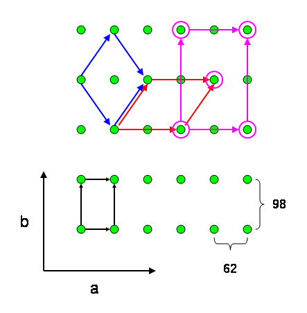
Figure 1. The action of matrix M on the original lattice of the (P212121 native) lego cell is shown. The original orthorhombic cell is shown in black. The monoclinic cell obtained after application of matrix M is shown in red. A cell reduction of the red unit cell results in the blue SeMet1 cell. The C-centered cell of the SeMet2 derivative is shown in pink. The view is along the original c axis.
Comparing Native and SeMet1 to SeMet2
Although it is rather obvious that the Native data is related to SeMet2 (there is a factor 2 in the a and b axis), it might not be entirely clear where the centring comes from. The presence of the centring operator becomes however clear when comparing the Niggli cells of the two Se-Met derivatives
Niggli cell SeMet1:
   Unit cell: (115.5, 115.6, 149, 90, 90, 115)
   Space group: P 1 1 21 (No. 4)

Niggli cell SeMet2:
   Unit cell: (115.6, 115.6, 148.9, 90, 90, 115.4)
   Space group: Hall:  C 2c 2 (x-y,x+y,z)
Since the Niggli cells of the derivatives are similar, the introduction of the centring is a direct result of the pseudo symmetric properties of the Niggli cells of the Selenium derivatives. A graphical depiction of the situation is shown in Figure 1.
The relations found between these various crystal forms can be practically relevant when attempting to perform molecular replacement against multiple crystal forms (Di Constanzo et al., 2003) or when performing multiple crystal density modification.
4. Availability
The program iotbx.explore_metric_symmetry is open source code included in the CCTBX.
5. Acknowledgements
We gratefully acknowledge the financial support of NIH/NIGMS through grants 5P01GM063210 and 5P50GM062412. Our work was supported in part by the US department of Energy under Contract No. DE-AC02-05CH11231.
6. References
- Andrews, L.C., Bernstein, H.J. & Pelletier, G.A. (1980). Acta Cryst. A36, 248-252.
- Billiet, Y. & Rolley Le Coz, M. (1980). Acta Cryst. A36, 242-248.
- Dauter, Z., Li, M. & Wlodawer, A. (2001). Acta Cryst. D57, 239-249.
- Di Constanzo, L., Forneris, F., Geremia, S. & Randaccio, L. (2003). Acta Cryst. D59, 1435-1439.
- Grosse-Kunstleve, R.W. (1999). Acta Cryst. A55, 383-395.
- Grosse-Kunstleve, R.W., Sauter, N.K. & Adams, P.D. (2004a). Acta Cryst. A60, 1-6.
- Grosse-Kunstleve, R.W., Sauter, N.K. & Adams, P.D. (2004b). Newsletter of the IUCr Commission on Crystallographic Computing 3, 22-31.
- Lehtio, L., Fabrichniy, I.,Hansen, T.,Schonheit, P.,Goldman, A. (2005). Acta Cryst. D61, 350-354.
- Le Page, Y. (1982). J. Appl. Cryst. 15, 255-259.
- Lebedev, A.A., Vagin, A.A. & Murshudov, G.N. (2006). Acta Cryst. D62, 83-95.
- Poulsen, J.-C.N., Harris, P., Jensen, K.F.& Larsen, S. (2001). Acta Cryst. D57, 1251-1259.
- Rutherford, J.S. (2006). Acta Cryst. A62, 93-97.
- Sauter, N.K., Grosse-Kunstleve, R.W. & Adams, P.D. (2006). J. Appl. Cryst. 39, 158-168.
- Skrzypczak-Jankun, E. ,Bianchet, M.A.,Mario Amzel, L. & Funk, M.O. Jnr, (1996). Acta Cryst. D52, 959-965.
- Zwart, P.H., Grosse-Kunstleve, R.W. & Adams, P.D. (2005), CCP4 Newsletter, 42, Winter 2005.