Daresbury Laboratory,
Daresbury,
Warrington
WA4 4AD, U.K.
m.d.winn@dl.ac.uk
ANISOANL is a new CCP4 program (available with version 4.1) which provides some simple tools for analysing ADPs. In this article, I will give an overview of these tools. Examples are taken from a 1.5A structure of barnase (PDB id 1a2p) and a 1.15A structure of myoglobin (PDB id 1a6g). For information on running the program, please see the program documentation. For information on obtaining the program, please see the CCP4 web pages.
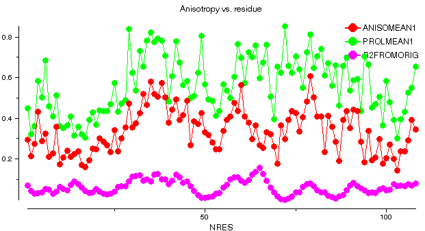
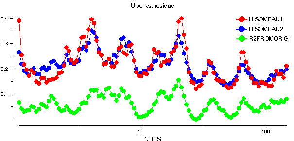
barnase: 1a2p
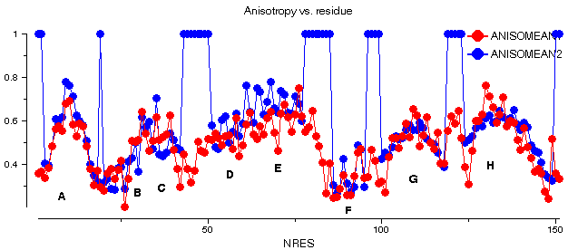
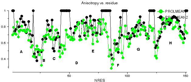
This graph shows some plots for chain A of barnase. ANISOMEAN1 is the anisotropy A, averaged over main chain atoms for each residue, while PROLMEAN1 is the prolate/oblate discriminator, similarly averaged. Most residues have an average anisotropy in the range 0.2 to 0.6 which is fairly typical. The value of PROLMEAN generally lies closer to A than to unity, implying a tendency towards prolate ellipsoids. R2FROMORIG shows the square of the distance from the centre of mass of the molecule.
Rosenfield et al. (1978) proposed a `rigid-body postulate' based on refined ADPs. Since interatomic distances within a rigid body are fixed, the difference in the projections of the ADPs of 2 atoms in a rigid body (the `Delta' value) must be zero. Note that this applies to all pairs of atoms in the rigid body, and not just bonded pairs. This is a necessary but not sufficient condition for rigid-body displacements. In any case, since proteins are never completely rigid, we can only identify possible quasi-rigid groups from low values of Delta for a set of atoms. Schneider (1996) has applied this approach to the protein SP445.
ANISOANL will produce a postscript figure giving Delta values between pairs of atoms, averaged over a number of bins. For example, using the main chain atoms of barnase, one gets the following figure:
barnase: 1a2p
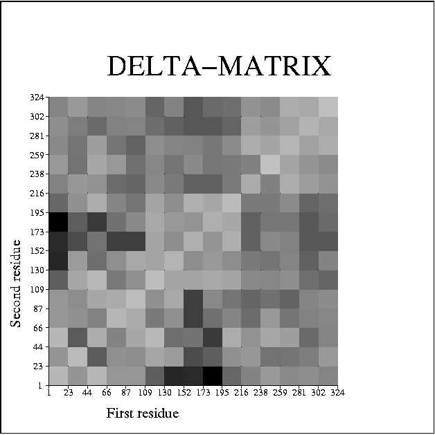
Light shading corresponds to low values of Delta, while dark shading corresponds to high values of Delta. Possible rigid-body behaviour is indicated by blocks of light shading. The blocks may or may not be contiguous along the protein chain. These plots are usually very noisy, but it is usually possible to discern some structure (perhaps with the help of the `Geophys' team!). In this example, it is possible to identify the three molecules of barnase that occur in the asymmetric unit (labelled as residues 1-108, 109-216 and 217-324). Thus it appears that the 3 molecules each move as a quasi-rigid body.
To analyse these results further, it is necessary to explicitly identify the three molecules as three rigid bodies. This is done via the TLSIN file, which in this case is:
TLS
RANGE  'A   3.' 'A 110.' MNCH

TLS
RANGE  'B   3.' 'B 110.' MNCH

TLS
RANGE  'C   3.' 'C 110.' MNCH
Each "TLS" record begins a new rigid group, consisting of the atoms specified in one or more "RANGE" records.
ANISOANL plots the distribution of Delta values for each rigid group, and for all pairs of atoms belonging to different rigid groups (the OFFDIAG plot):
barnase: 1a2p
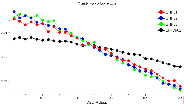
The distribution is similar for each putative rigid group, while the OFFDIAG plot is skewed towards higher values of Delta. This implies that pairs of atoms within a molecule satisfy the rigid body postulate better than pairs of atoms from different molecules.
A second example, which looks at the internal structure of a single molecule rather than several whole molcules, is given by the 1.15A structure of a myoglobin-CO complex (PDB id 1a6g). The plot of the Delta matrix looks like:
myoglobin-CO: 1a6g
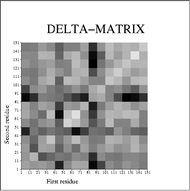
Again there is a lot of noise, but it is possible to pick out possible pseudo-rigid regions at residues 1-21, 21-41, 51-81, 81-101 and 101-151. In fact, these regions correspond closely to helices A (residues 3-18), B and C (20-35,36-42), D and E (51-57,58-77), F (86-95) and G and H (100-118,124-149) respectively. Looking at the inter-helix Delta values, helix F stands out in particular as having large Delta values, and thus not being part of any larger pseudo-rigid group. It appears that helices, or pairs of helices, form the relevant units for describing large scale displacements in myoglobin.
I have done this for the barnase structure treating each molecule as a separate TLS group (i.e. using the TLSIN file given in the previous section). The success of the fitting can be assessed by comparing the equivalent isotropic displacement parameter, the anisotropy and the prolate/oblate discriminator derived from the TLS parameters (labelled UISOMEAN2, ANISOMEAN2 and PROLMEAN2) to those derived from the refined ADPs. This is shown for chain C of barnase (this shows the best fit, though chains A and B are similar):
barnase: 1a2p
barnase: 1a2p
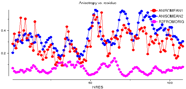
barnase: 1a2p
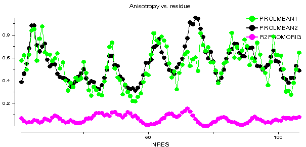
The fit is fairly good, and thus TLS provides a good first-order description of the refined ADPs. The discrepancies show, however, that there is some detail unaccounted for by the pseudo-rigid body description.
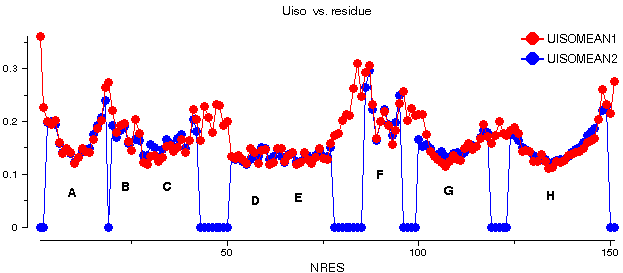
I have also fitted TLS parameters to the myoglobin structure. Following the results of the Delta-matrix analysis given above, I have used 6 TLS groups based on the alpha helices, with helices D and E being treated as a single group, and likewise helices G and H:
TLS
RANGE  'A   3.' 'A  18.'  FIT  MNCH

TLS
RANGE  'A  20.' 'A  35.'  FIT  MNCH

TLS
RANGE  'A  36.' 'A  42.'  FIT  MNCH

TLS
RANGE  'A  51.' 'A  57.'  FIT  MNCH
RANGE  'A  58.' 'A  77.'  FIT  MNCH

TLS
RANGE  'A  86.' 'A  95.'  FIT  MNCH

TLS
RANGE  'A 100.' 'A 118.'  FIT  MNCH
RANGE  'A 124.' 'A 149.'  FIT  MNCH
The resultant TLS parameters are used to calculate ADPs which are compared to the refined ADPs as follows:
myoglobin-CO: 1a6g
myoglobin-CO: 1a6g
myoglobin-CO: 1a6g
The fit is clearly very good for both Uiso and the anisotropic components (residues with UISOMEAN2 = 0 and ANISOMEAN2 = PROLMEAN2 = 1 are those not included in any TLS group).
A more detailed rigid-body analysis of 1a6g was given by Vojtechovsky et al. (1999) who fitted TLS parameters to helices E and F, as well as to the heme group. They concluded on the basis of this fit that helix F and the heme group had ADPs consistent with rigid-body displacements, while helix E is less well described by a rigid body model.
These authors gave TLS parameters for helix F (and the heme group) which can be compared with the present results (analysis of the TLS tensors was done using the CCP4 program TLSANL):
                  T axes and eigenvalues (A**2)    L axes and eigenvalues (deg**2)

                     [-0.20, -0.25,  0.95] 0.18      [ 0.07, -0.16,  0.98]  27.2
Vojtechovsky et al.  [ 0.06, -0.97, -0.24] 0.09      [ 0.19, -0.97, -0.17]   4.3
                     [ 0.98,  0.01,  0.21] 0.08      [ 0.98,  0.20, -0.04]   0.6

                     [-0.26, -0.30,  0.92] 0.21      [ 0.15, -0.11,  0.98]  34.1
This study:          [ 0.00, -0.95, -0.31] 0.09      [ 0.35, -0.92, -0.15]   6.7
                     [ 0.97, -0.08,  0.25] 0.15      [ 0.93,  0.37, -0.10]  -2.0
There are some discrepancies due to differences in the atom selection
used for the TLS groups, but the overall picture is the same. (The negative
value for the 3rd eigenvalue of L is unphysical, but allowed by the
fitting procedure, and illustrates that there is some over-fitting.) In particular,
there is a dominating libration parallel to the Z axis, and approximately
parallel to the helix axis. These axes may be displayed using the
AXES
option of TLSANL.
In the version released with 4.1, ANISOANL can only be run from the command line. However, a task interface for ccp4i is in preparation, and will be made available soon. For full details of the program, see the distributed documentation.