 , (1.1)
Maximal Likelihood refinement. It works, but why? (Seminar notes).
by Vladimir Y.Lunin
a,b & Alexander G.Urzhumtseva(aLCM3B, University of Nancy, France, e-mail: sacha@lcm3b.u-nancy.fr;
bIMPB RAS, Pushchino, Russia, e-mail: lunin@impb.psn.ru)
Recently the Crystallographic Laboratory (LCM3B) of the University of Nancy, France, has organized a seminar on crystallographic methodology. One of the purposes of this seminar is to analyze some basic crystallographic approaches which are not always clear presented in the current literature. Such clarification becomes more and more important with increasing the number of scientists who does not have enough background intheoretical crystallography but rather uses it as a "black box" tools for their researches.
Last years (Bricogne & Irwin, 1996; Pannu & Read, 1996; Read, 1997; Murshudov et al., 1997; Pannu et al., 1998) the so called maximal likelihood refinement (MLR) had been proven as a useful tool, which significantly extends the possibilities of refinement. Nevertheless, the reasons for this success are not well explained in the literature. Another general problem is that in probabilistic or in statistical methods the authors of the papers quite rare clearly explain which are the random variables, which probability they are talking about and which statistical hypothesis is testing. An essay to get a more materialistic background for the MLR was a goal of the one of methodological seminars in Nancy. This paper contains a brief notes from this seminar.
1. Conventional refinement
2. Likelihood based refinement. I. Experimental errors.
3. Likelihood based refinement. II. Incomplete models.
4. How to calculated the likelihood value
5. Likelihood maximization.
6. Analysis of RML residual.
7. Discussion
8. References
Appendixes
A1. Structure factors formula
A2. Randomly generated additional atoms
A3. The likelihood corresponding to the partial model
A4. Modified Bessel functions
A5. Modified observed magnitudes
1. Conventional refinement.
In order to have the situation maximally transparent, we do not consider below the problem in its most general form, but study simplified cases which still hold the main features of the problem. In particular, we suppose that the atomic coordinates only must be defined, while atomic scattering factors and temperature movement parameters are known precisely.
The goal of the conventional structure refinement may be formulated as follows:
Conventional refinement
The goal of the refinement is to find the atomic coordinates resulting in structure factors magnitudes which are as close as possible to the observed magnitudes.
When we say that atomic coordinates result in some structure factors (s.f. in what follows) we mean that there exists a s.f.-formula (Appendix A1) which allows to calculate s.f. provided the coordinates are known. Mathematically the conventional refinement goal may be formulated as a minimization problem, e.g. as follows
 , (1.1)
where the calculated magnitudes depend on atomic coordinates by means of (Appendix A1, (A1.1)) and w(h) are some weights. Eventually, other criteria can be used as a measure of discrepancy between two data sets instead of the least-square criterion (1.1). The conventional R-factor or R-free factor may serve as a measure of the refinement success.
This goal seems to be quite reasonable when the model is complete and the s.f.-formula is precise, i.e. when the structure factors magnitudes calculated with the use of the full set of exact atomic coordinates are equal to the corresponding observed values. The goal is not so evident in some other cases when, for example, the observed magnitudes contain experimental errors or the model is incomplete (e.g., solvent atoms are not included into the model). In such situations the s.f. magnitudes calculated with the exact coordinates of atoms are not equal, in general, to the observed magnitudes. So, the conventional refinement fits the calculated s.f. magnitudes to wrong values.
To reveal the differences in these two kinds of errors we consider them separately. The discussion how they may be combined may be found in (Pannu & Read, 1996).
2. Likelihood based refinement. I. Experimental errors.
Obviously, to take into account the experimental errors it is necessary to have some information about them. Sometimes this information may be introduced as a probability distribution for the errors values. For example, we can suppose that the errors
e(h) in the magnitudes Fobs(h) are independent random variables distributed in accordance with the Gaussian law with zero mean and the known standard deviation s(h): .
(2.1)
The parameters
s(h) characterize the instrument precision and are external for the refinement information. We will not discuss here how these values may be estimated in practice.Supposing the values
s(h) are known, we can estimate for every trial set of atomic coordinates {rj} how high would be chances to obtain again in the experiment the same set of Fobs(h) values, would the quantities obtained in experiment differ from Fcalc(h;{rj}) by errors e(h) only. In other words, we can calculate the probability that the measured magnitudes are just "the calculated ones plus random errors, distributed as (2.1)":![]()
 , (2.2)
where the product is calculated over all experimentally obtained magnitudes.
For different trial sets of atomic coordinates this probability is different. If it is too small, it is reasonable to reject the considered coordinates, as the differences between calculated and observed magnitudes fall outside our assumptions about possible errors. As a generalization of this idea, it is reasonable to consider as the best coordinates those which maximize this probability.
ML-refinement. I.
The goal of the refinement is to find the atomic coordinates {rj} which maximize the probability to reproduce in the X-ray experiment the set of experimental values {Fobs(h)} provided the experimentally obtained magnitudes differ from the calculated ones by the errors distributed as (2.1).
It must be emphasized that this idea is just a "common sense" rule. It can not be "proven" formally.
The suggested MLR-principle is nothing, but the maximal likelihood principle which is broadly used in the Mathematical Statistics. In the considered case the probability (2.2) is called as the likelihood corresponding to statistical hypothesis:
e(h). These errors are independent and distributed in accordance with the Gaussian law with zero mean and known standard deviations s(h).Hypothesis H(r1,…,rNfull)
The experimentally determined Fobs(h) values differ from Fcalc(h;r1,…,rNfull) by random experimental errors
The maximization of (2.2) is equivalent to the minimization:
 . (2.3)
We see that in the considered case the MLR refinement is formally equivalent to the conventional refinement (1.1) with appropriately chosen weights w(h)=1/s
2(h). So the conventional refinement may be considered as a type of ML-refinement. Nevertheless a more sophisticated probabilistic modeling of the differences between calculated and observed magnitudes may result in penalty functions different from (2.3) .3. Likelihood based refinement. II. Incomplete model.
We consider now another case when Fobs(h) values are supposed to be measured precisely (or the errors may be considered as negligible ones), but the model is incomplete. We refer to this model as a partial one.
For the clarity we write the formulae below for nc/s reflections. The necessary corrections for centric reflections are straightforward.
The s.f. magnitudes calculated with the exact atomic coordinates of a partial model are not equal, in general, to the observed magnitudes, but differ from them in unknown quantities corresponding to the absent atoms. The problem could be overcome could we have a possibility to get from an experiment s.f. magnitudes corresponding to the partial structure and adjust to them the values calculated with the partial model. As this is not possible in general, an alternative way could be to introduce some corrections into the measured magnitudes values compensating the absence of a part of atoms in the model. We will show below that ML refinement may be considered from this point of view too.
While the known true atomic position for a part of structure do not allow to reproduce the structure factor magnitudes Ffull(h) correctly, their are some chances to get these values if the absent atoms are added to the model with randomly chosen coordinates (Appendix A2). One can expect that it would be less chances to reproduce Ffull(h) correctly when the randomly chosen atomic positions are added to a wrong partial model than to the exact one. Therefore, it seems reasonable to consider the partial model coordinates which provide maximal chances to improve the model when generating the coordinates for absent atoms randomly as the best ones. Again, this idea is nothing but the maximal likelihood principle, which now is applied to a different type (in comparison with Sec.2) of statistical hypotheses.
We define now the goal of the refinement as the following one.
ML-refinement. II.
We look for the set of partial model coordinates which maximizes the chances to make calculated magnitudes equal to the observed ones when completing the partial model by Nadd additional randomly placed atoms.
In a more formal way the goal may be formulated as the following: under the hypothesis that the experimental magnitudes may be reproduced by means of adding randomly of Nadd atoms to the partial model, maximize the likelihood (Appendix A3) varying the atomic coordinates of the partial model.
It is worthy of noting that as many other statistical approaches, the maximal likelihood principle is just a "common sense" principle. It can not be "proven", and all its "good properties" reveal themselves "in mean", when it is applied regularly. In other words, the maximal likelihood principle works statistically and does not guaranty the correct choice when being applied to a single particular object.
It must be emphasized that the ML-refinement is not just a new penalty function. It changes the goal of refinement. We do not try any longer to fit the calculated magnitudes to the observed ones, but try to maximize chances for the further improvement of the model. As a consequence, the conventional R-factors (as well as R-free) may, in general, increase their values in the course of the likelihood maximization.
4. How to calculated the likelihood value.
In order to realize the goal of the ML-refinement we must have a possibility to calculate the likelihood value provided coordinates of the partial model are known. The usual way includes the following steps:
a) derive the joint probability distribution (j.p.d.) for magnitudes and phases of the calculated structure factors;
b) derive the marginal probability distribution for the calculated s.f. magnitudes by means of the integrating of the j.p.d. over the phases;
c) obtain the likelihood value by replacing the Fcalc(h) with Fobs(h) in the formula for the magnitude probability distribution.
4.1. Joint probability distribution of real and imaginary parts of a structure factor.
The simplest way to get j.p.d is based on The Central Limit Theorem of the Theory of Probabilities. This theorem states that the sum of independent (or "slightly" dependent) random variables is distributed in accordance with the Gaussian distribution. This means that we know in advance the shape of distribution and all what must be defined is a small number of the distribution parameters.
We consider first one nc/s structure factor and study the j.p.d. of its real and imaginary parts. In the general case the two-dimensional Gaussian distribution is defined by five parameters, namely mean values and dispersions corresponding to every of the two coordinates and the correlation coefficient between these coordinates. However, in our case it is defined, in fact, by only one parameter b (Srinivasan & Parthasarathy, 1976) which is equal to Nadd*g(h):
 . (4.1)
Here A and B are real and imaginary parts of a structure factor corresponding to the mixed model (the known partial model plus random atoms), they both are random variables. Apart and Bpart corresponds to the partial model, they are some defined values and not random variables! The parameter b is defined as <Aadd2>=<Badd2>=b/2, Aadd and Badd correspond to the additional atoms and <...> means the expected value of the corresponding random variable.
4.2. Joint probability distribution of magnitude and phase of a structure factor.
The j.p.d. of the magnitude and phase can be obtained simply by rewriting in "polar coordinates" the Gaussian distribution derived above:
 .
(4.2)
Here Fexp[ij ] is a random structure factor corresponding to the mixed model, and Fpartexp[ij part] is those corresponding to the partial model; the latter is some fixed (not random) value.
4.3. Marginal distribution for s.f. magnitude. The likelihood.
Now we can derive a marginal distribution for the magnitude by integration of j.p.d. "magnitude-phase" over phases.
 (4.3)
(4.3)
and calculate the marginal likelihood L=P{F = Fobs}, provided a single experimental observation is taken into account
 .
(4.4)
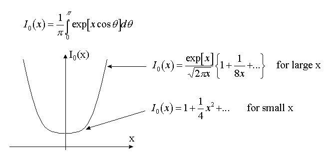
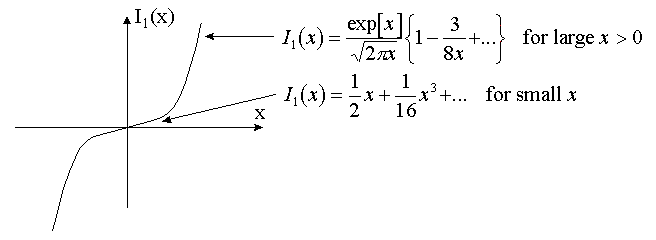
Here Io(t) stands for the modified Bessel function of the zero order (Appendix A4).
In practice we have, obviously, observed magnitude values for many reflections. Therefore, the likelihood must be calculated using all these observations. The Central Limit Theorem allows to get j.p.d. of all magnitudes and phases, corresponding to the mixed model. This distribution is defined by the mean values and the full set of second order moments calculated for the real and imaginary parts of the structure factors. Nevertheless, it is not possible, in general, to perform in a close form the integration over the phases to get marginal distribution for s.f. magnitudes. A possible way is to neglect the correlations between different s.f. and to consider different complex structure factors as independent random variables ("diagonal approximation"). In this case the probability distribution for a set of s.f. magnitudes is just the product of distributions corresponding to individual reflections and the likelihood is
 (4.5)
(4.5)
We remind that Fpart(h) here depends on the model coordinates {rj}, while Fobs(h) and b(h) are known values.
As the logarithm is a monotonically growing function, any function and its logarithm have minima or maxima simultaneously. This means that in our case we can replace the likelihood maximization by the maximization of its logarithm which computationally is much more convenient

 . (5.1)
Additionally, it is convenient to skip the first sum which is independent on the partial model coordinates and to maximize the so called Logarithm Likelihood Gain (LLG) value
 .
(5.2)
The maximization of the LLG is equivalent to the minimization of
![]()
, (5.3)
so ML-refinement is nothing but minimization of RML residual and all relevant minimization methods may be used.
Let's analyze more thoroughly a particular item in the last sum as a function depending on Fpart(h):
 .
(6.1)
For large F values I0 grows near exponentially, so the second term grows near linearly and the whole yh(F) function grows as a quadratic function. For small F values we have
 .
(6.2)
This shows that the function yh(F) has different behavior depending on the ratio of (Fobs)2 to b .
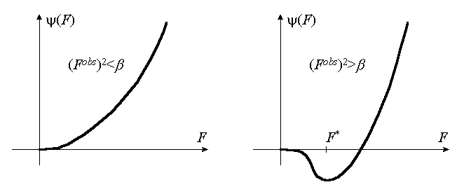
For relatively small Fobs (the ratio is smaller than 1) the minimum of yh(F) is attained for F=0. This means that in order to minimize the RML
, the calculated s.f. magnitudes Fpart(h;{rj}) for relatively week reflections must be fit to zero. If Fobs are relatively large (the ratio (Fobs)2/b is larger than 1), then the function yh(F) has nonzero minimum F* and in order to minimize RML the Fpart(h;{rj}) values in the corresponding members in the sum must be fit to F*(h).In other words, the ML refinement is similar to the minimization of a simplified residual
 (6.3)
(6.3)
where F*(h) may be thought as modified observed values.
The modified magnitudes F*(h) are equal to zero for week reflections (with (Fobs)2<b ). For relatively strong reflections the modified value F*(h) are found from the condition
 ,
(6.4)
and have nonzero values. The dependence F*(Fobs) is shown for different b at the figure below (see Appendix 5 for details). It is worthy of noting that the modified value F*(h) is always less than the experimental one.
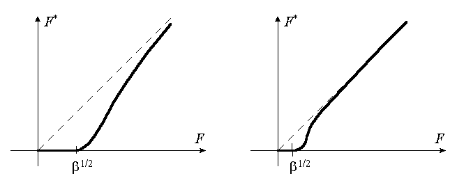
It must be noted that the scale of the modification of the observed values depends on the value of b parameter which reflects the completeness of the current model. If (in the considered situation) the number of atoms absent in the model is big, then b value is high and many modified values F*(h) are taken as zero ones, while other may be significantly less than Fobs(h) values. If the number of absent atoms (and b ) is small, then deviations F*(h) from Fobs(h) are small and ML-refinement coincides with the conventional one.
Some additional issues are worthy of noting.
1. It was shown that the ML-refinement may be considered as an attempt to fit the calculated (from an incomplete model) structure factors magnitudes to some modified experimental magnitudes. The modification consists in reduction of values of structure factor magnitudes; week magnitudes becomes zeros but are not excluded from the refinement. The cut-off level and the degree of reduction depend on the value of the parameter b , in other words, on the number of absent atoms in the considered case. If the relative number of absent atoms is relatively small, the modified F*(h) values are close to Fobs(h) and ML-refinement is reduced to the conventional refinement.
2. In the considered case the j.p.d. for magnitude and phase of s.f. depends on one parameter b . In a more general situation it may depend on two parameters a and b

which reflect the accuracy of s.f.-formula and must be defined in advance. The procedure based on the maximization of a marginal likelihood corresponding to the test set of reflections may be used for these purposes (Lunin & Skovoroda, 1995; Read, 1997). It was discussed also (Lunin & Skovoroda, 1995) that this distribution is valid for many cases of errors and therefore the considerations done above are valid in many other applications.
3. The simplified residual may be written in a more close to RML form if the weights are applied which are equal to yh’’(F*).
4. To introduce stereochemical or energy restraints into the refinement the usual penalty functions may be added to RML
residual.
This work was partially supported (VYL) by RFBR grant 97-04-48319 and by CNRS Fellowship.
Bricogne, G., Irwin, J. (1996) Macromolecular Refinement: Proceedingof the CCP4 Study Weekend, E.Dodson, M.Moore, A.Ralph & S.Bailey, eds., pp.85-92. Warrington : Daresbury Laboratory.
Lunin, V.Yu. & Skovoroda, T.P.(1995). Acta Cryst. A51, 880-887.
Murshudov, G.N., Vagin, A.A. & Dodson, E.J. (1997). Acta Cryst. D53, 240-255.
Pannu, N.S., Murshudov, G.N., Dodson, E.J. & Read, R.J. (1998) Acta Cryst. D54, 1285-1294
Pannu, N.S. & Read, R.J. (1996). Acta Cryst. A52, 659-668.
Read, R.J. (1997) In Methods in Enzymology, Academic Press, San Diego., C.W.Carter, Jr., R.M.Sweet, eds., 277, part B, 110-128.
Srinivasan, R. & Parthasaraty, S. (1976). Some Statistical Applications in X-ray Crystallography. Oxford: Pergamon Press.
Appendixes.
We suppose that the structure factors are connected with the atomic coordinates by means the s.f.-formula
 ,
(A1.1)
here
![]() are atomic coordinates; h
is a reciprocal space vector;
are atomic coordinates; h
is a reciprocal space vector; ![]() are known functions which include both scattering and temperature factors
and atomic occupancies;
are known functions which include both scattering and temperature factors
and atomic occupancies; ![]() is
calculated over all atoms included into the model.
is
calculated over all atoms included into the model.
In our consideration the values of the magnitudes and phases of calculated s.f. are functions which depend only on the coordinates of the atoms included into the model.
1. Conventional refinement
A2. Randomly generated additional atoms
We consider as the object of the refinement a current partial model which includes Npart
atoms only while Nadd atoms (solvent atoms e.g.) are absent:Nfull=Npart+Nadd
;![]() ,
(A2.1)
,
(A2.1)
where
![]() ;
(A2.2)
;
(A2.2)
r1,. . ., rNpart are coordinates of atoms which are included into the current model (these coordinates are known approximately), while u1,. . ., uNadd are totally unknown coordinates of the atoms absent in the model.
We consider here the coordinates of additional atoms u1,. . . uNadd as random variables distributed uniformly in the unit cell and suppose that all atoms are of the same type and have the same scattering factor g(h). So
 ,
(A2.3)
where {u
j} are the coordinates of additional atoms. (More sophisticated hypotheses may be considered in a similar way which take into account an extra information about possible positions of additional atoms.)In such the case in the identity
![]() ;
(A2.4)
;
(A2.4)
![]() is a random (complex)
variable;
is a random (complex)
variable;
![]() is a determined
(non-random) value which depends on the partial model coordinates r1,.
. .,rNpart.
is a determined
(non-random) value which depends on the partial model coordinates r1,.
. .,rNpart.
The “mixed model” structure factor ![]() is now a random variable (as it includes a random part
is now a random variable (as it includes a random part ![]() ), but its probability
distribution is different for different sets of coordinates r1,.
. .,rNpart of the partial model.
), but its probability
distribution is different for different sets of coordinates r1,.
. .,rNpart of the partial model.
BACK TO: 3. Likelihood based refinement. II. Incomplete model.
A3. The likelihood corresponding to the partial model
The likelihood value corresponding to some statistical hypothesis may be considered as the probability to reproduce the experimentally observed data under this hypothesis (to be mathematically correct, when the observations correspond to continuous random variables it is necessary to speak about probability distribution function values rather then probabilities).
In the studied case we can formulate the statistical hypotheses as follows:
Statistical hypothesis H({r1,. . . , rNpart})
The correct structure may be obtained by adding of Nadd
atoms with randomly generated coordinates u1,. . ., uNadd to the Npart atoms with the known positions r1,. . . , rNpart.
Every of these hypothesis is specified by the set of the partial model coordinates {rj}. As a consequence, the problem of the choice of the particular values of these coordinates may be formulated as the problem of the choice of the hypothesis which is the most consistent with the experimental data.
Under the hypothesis H, the values of calculated (with the use of s.f.-formula A3) s.f. magnitudes are random variables (as they depend on random {uj}) and we can speak about the probability for these variables to have some particular values.
For every hypotheses H, we can define the probability of the calculated s.f. magnitudes to be equal to the observed ones:
L(H)=Probability{Fcalc(h) = Fobs(h) for h from S},
where S is the set of experimentally measured intensities. This value L(H) is called the likelihood corresponding to this hypothesis. As the hypothesis is specified by the partial model coordinates, the likelihood value L(H) is the function depending on the model coordinates:
L(H)=L(r1,. . ., rNpart) =
Probability{u}{Fcalc(h;{rj}+{uj}) = Fobs(h) for h from S},
where the probability appears due to random coordinates {uj}.
Naturally, this probability varies with different hypotheses (i.e., for different partial model coordinates) and the maximal likelihood principle suggests to accept the hypothesis which possesses of the maximal likelihood value, i.e. to accept values of the partial model coordinates which maximize the L(r1,. . ., rNpart).
BACK to: 3. Likelihood based refinement. II. Incomplete model.
BACK to: 4. How to calculated the likelihood value
A5. Modified observed magnitudes
The modified values F*(h) may be found from the condition
![]() ,
(A5.1)
,
(A5.1)
i.e. from the equation
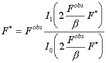 .
(A5.2)
The ratio of the first and zero order modified Bessel functions has the following properties:
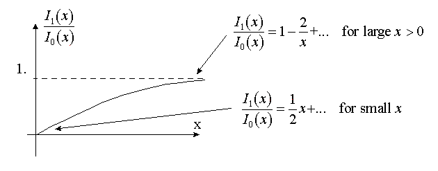
So, depending on the value (Fobs)2/b two cases can exist:
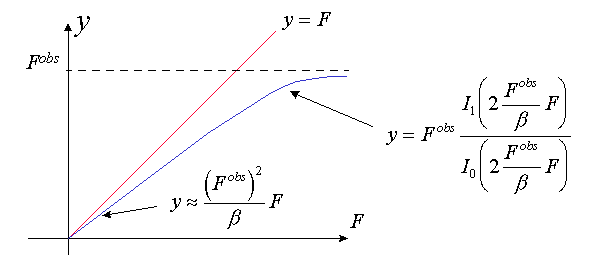
The case (Fobs)2<b . The equation y ’(F)=0 has the only solution F*=0.
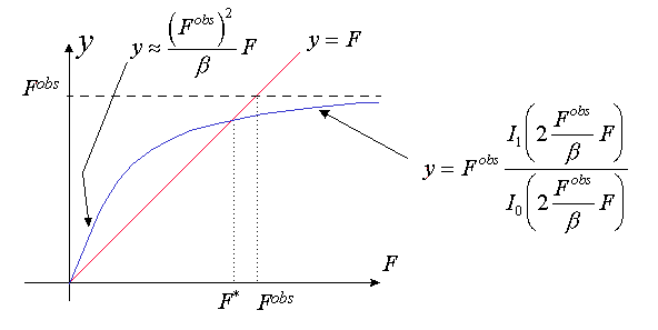
The case (Fobs)2
>b . The equation y ’(F)=0 has a nonzero solution F*.It is easy to see that in this case F
*<Fobs.BACK to: 6. Analysis of RML residual.