by
Valérie Biou
Laboratoire de Cristallographie Macromoléculaire, Institut de Biologie
Structurale
41 avenue des Martyrs
F-38027 Grenoble cedex, France
and European Synchrotron Radiation Facility, BP 220, F-38043 Grenoble cedex
France.
e-mail biou@ibs.fr
Many structures have been solved using MAD data during the last few years, and
their number is increasing exponentially. The aim of this paper is to give a
practical approach to MAD, and in particular to the use of MIR programs to
phase MAD data, and to discuss the limitations and advantages of the method.
In the presence of anomalously scattering atoms in the protein crystal, one can
use two types of signal to calculate phases from a diffraction data set : (i)
dispersive difference signal : due to the contribution of F'a to the structure
factor, the intensity of a given reflection changes with the wavelength. (ii)
anomalous signal : the intensity of symmetry related reflections is different
due to the contribution of F"a (fig 1).
These signals can be used in a multiple wavelength dispersion (MAD) experiment
with tuneable synchrotron radiation, so that both the dispersive and anomalous
differences are maximised. This takes at least 3 wavelengths, which we shall
define as follows :  1 is measured at the minimum of f', i.e., the
inflection point of the fluorescence spectrum ; 2 is taken at the
maximum of f" (and of the fluorescence spectrum) ; 3 is taken on the
high energy side of the spectrum. Thus, that 1 and 3
maximise the dispersive difference signal, and 2 maximises the
anomalous signal. A fourth wavelength, remote on the low energy side of the
edge, can also be useful.
1 is measured at the minimum of f', i.e., the
inflection point of the fluorescence spectrum ; 2 is taken at the
maximum of f" (and of the fluorescence spectrum) ; 3 is taken on the
high energy side of the spectrum. Thus, that 1 and 3
maximise the dispersive difference signal, and 2 maximises the
anomalous signal. A fourth wavelength, remote on the low energy side of the
edge, can also be useful.
The advantages and disadvantages of MAD have been explained elsewhere (see for
example Reid, 1996). Briefly, it is obvious that one overcomes anisomorphism
problems between native and derivative by using MAD. One can collect three data
sets on a single, flash frozen crystal containing an appropriate element. On
the other hand, the anomalous signal is generally much less intense than the
isomorphous signal for the same element. Just consider the example of the
replacement of sulphur by selenium in selenomethionine. The K edge of selenium
contributes 10 electrons at the maximum dispersive difference, whereas it gives
18 electrons isomorphous signal compared to sulphur. Even for such a light atom
as selenium, the isomorphous difference will be roughly twice as large as the
dispersive difference. In the case of mercury, the difference between the
anomalous and the isomorphous contributions is even larger.
Therefore, the problem is to measure small differences between large figures.
This has been said before, but it should be stressed : it is vital for a MAD
experiment to get accurate measurements. Synchrotron beamlines have been
developed that allow to do this in a shorter and shorter time, and in the next
few months there should be less shortage of beam time for MAD (see A.W.
Thompson's paper in this issue).
Data
collection and its preliminaries
In order to properly plan an experiment, it is important to evaluate the
theoretical signal one can expect to obtain from a given heavy atom
derivative: these are the dispersive ratio, and the anomalous ratio, which give
the proportion of the maximum anomalous or dispersive signals vs. the total
scattering power of the macromolecule. Dispersive ratio =

Anomalous ratio =
 where
where
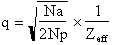 .
Na = number of anomalously diffracting atoms in the unit cell, Np = number of
protein atoms, and Zeff = 6.7 electrons for a protein crystal (mean effective
normal scattering on protein atoms), 1, 2 and 3
are defined as in the introduction. In practice, a signal of 2.5% with very
good data may be enough for phasing. 3.5 to 4% gives a good signal.
.
Na = number of anomalously diffracting atoms in the unit cell, Np = number of
protein atoms, and Zeff = 6.7 electrons for a protein crystal (mean effective
normal scattering on protein atoms), 1, 2 and 3
are defined as in the introduction. In practice, a signal of 2.5% with very
good data may be enough for phasing. 3.5 to 4% gives a good signal.
It is just as essential to have good knowledge of your crystals : mosaicity,
resolution, diffracting power. Too high a mosaicity will make the data harder
to integrate, and reduce the signal to noise ratio. MAD structures have been
solved with mosaic crystals (up to 1deg. as defined in DENZO), but 0.4deg. or
less gives better signal. If the crystal diffracts to high resolution, it is
worth spending more time to collect high resolution at three wavelengths, to
get accurate experimental phases at higher resolution. This can be achieved if
the crystal diffracts strongly : the anomalous signal does not decay with
resolution, but if the spot intensities become too low, the measurements will
be more noisy, hindering the extraction of the anomalous signal.
It is essential to measure a fluorescence spectrum on your crystal ( or
2 with 2 perpendicular crystal orientations). The absorption edge can shift due
to anisotropy of the heavy atom chemical environment. This will determine the
strength and position of the fluorescence spectrum and will allow you to decide
at which wavelengths to collect. In case of a beam reinjection during the
course of the measurements, it is wise to collect a fluorescence spectrum
again.
The second step is to collect one image to determine the crystal orientation.
From this, one can run a data collection strategy program in order to
plan how much data needs to be collected. We routinely use Andrew Leslie's
STRATEGY option in MOSFLM (Leslie, 1996). From a given crystal orientation, it
gives the most convenient rotation range to run and predicts the expected
completeness, both for individual reflections and for Bijvoet mates. If the
crystal can be oriented so that it rotates around a mirror axis, it is better
to do so, as it allows to collect Bijvoet mates in the same image. In the case
where it is necessary to collect data from an additional crystal, the program
gives the best rotation range to complete the datasets. Once you have set up
the strategy and the best exposure time, start the actual data collection, and
measure 3 wavelengths, four if possible.
Finally, it is important to integrate and scale data carefully. A first run can
be done on the first wavelength, while it is being collected. It will give
information about the data quality and the anomalous signal to be expected from
the whole data set. Several integration and scaling runs are usually necessary
in order to get the best out of the data set (see P.R. Evans's contribution in
this issue).
Both phasing systems imply the location of heavy atoms positions in the
unit cell. This can be done using Patterson maps or direct methods. Three types
of Patterson maps can be used : dispersive difference Pattersons between two
wavelengths, or anomalous difference Patterson for one wavelength, or a
Patterson map calculated using the Fa's derived from the algebraic method (see
below). This last method seems to be the one that gives the least noisy
Pattersons, because systematic errors have been removed before. Similarly, the
same types of differences can be used in direct methods to solve the heavy atom
structure when the number of heavy atoms is too high (Bertrand et al.,
1997). This is probably going to be common practice in the near future, as
it will allow to phase larger and larger structures with MAD. Starting from the
location of heavy atoms, the next step is then to refine those and calculate
phases. Two types of methods are available for phasing MAD data.
The first method used to phase a novel structure using MAD data (Guss et
al., 1988), is based on the algebraic derivation of phases using a set of
linear equations (Karle, 1980). This method allows to derive accurate values
for the heavy atom structure factors (Fa), and gives an elegant solution of the
phase problem. However, though it is being made more user friendly (Wu and
Hendrickson, 1996), it has long been difficult to use, in particular because it
required a careful bookkeeping for equivalent reflections. It works on
unmerged, scaled individual reflections.
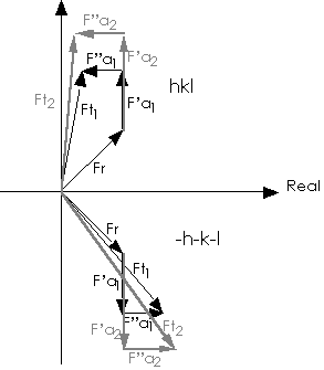
Figure 1 Vectorial representation of structure factors in the presence of
anomalous scatterers.
Subscripts 1 and 2 refer to two different wavelengths. Ft = total structure
factor for reflection hkl.; Fr = contribution from the non anomalously
scattering atoms;
F'a = contribution from the real part of anomalously scattering atoms;
F"a = contribution from the imaginary part of anomalously scattering atoms;
Ft=Fr+F'a+iF"a.
From fig 1, it is visible that the different wavelengths can be considered as
different heavy atom derivatives, and that multiple isomorphous replacement
phasing methods should be usable in this context. Ramakrishnan et al.
(1993) were the first to use an MIR program to solve a new structure using
MAD data. Last year, about half the structures solved using MAD data were
phased using an MIR program. It is more familiar to most protein
crystallographers, and it allows to easily bring together all sorts of phasing
information. A number of different programs can be used to do this, the most
popular being probably MLPHARE (Otwinowski, 1991).
All of those programs refine the heavy atom positions and temperature factors,
and refine phases against the lack of closure error. Most of the programs
available (see Table I and Ramakrishnan and Biou (1997)) rely on a reference
wavelength data set as the "native", and use the dispersive differences between
this reference wavelength and the others, as well as the anomalous differences
for all data. The differences lie in the statistical description of the phase
and amplitude spaces. MLPHARE and the maximum likelihood option of PHASES use a
maximum likelihood description of the phase space, thereby implying that most
of the error comes from the phases and not from the amplitudes. On the other
hand, SHARP uses a maximum likelihood description of the whole complex space,
both amplitudes and phases. For a better description, see Eric de la Fortelle's
paper in this issue. X-PLOR also offers a MAD phasing option (Burling et
al., 1996).
program       author         distribution        usage                principle
mlphare       Z.Ottwinovski  ccp4 suite      1 reflection     choose one wavelength as
(Otwinowski,                 , Daresbury   file,  1 list of   "native" ; refines heavy
1991)                                           atomic             atom parameters
                                              scattering      (different occupancy for
                                                factors          real and anomalous
                                                              parts), based on maximum
                                                               likelihood on the phase
                                                                       circle.
phasit        W. Furey       phases             several       choose one wavelength as
(Furey and                   suite,        reflection files   "native" ; refines heavy
Swaminathan,                 author            ; atomic        atom parameters against
1997)                                         scattering           origin-removed
                                              factors are        patterson, or using
                                              entered as         maximum likelihood,
                                              parameters        similarly to mlphare.
madmrg +      T.             author          madmrg merges    choose one wavelength as
heavy         Terwillinger                      all MAD       "native" ; refines heavy
(Terwillinge                               reflections into    atom parameters against
r, 1994b;                                   a "SIRAS"-like         origin-removed
Terwillinger                                data set. heavy     patterson;
one single
, 1994a)                                     refines heavy           occupancy.
                                            atom parameters
                                            and calculates
                                                phases.
sharp (de     E. de la       author         http interface     no reference wavelength
la Fortelle   Fortelle,                        with user        ; refines heavy atom
and           G. Bricogne                    friendly data        parameters using
Bricogne,                                     input.
One       anisotropic B factors
1997)                                      reflection file.    and maximum likelihood
                                                                in the whole complex
                                                                       space.
x-plor
V     A. Brunger     x-plor           distributed     still under development.
3.8.5                        package,      template macros,   choose one wavelength as
(Burling et                  Yale               merged                "native"
al., 1996)                   university     reflection file
Table
I Some of the programs which can be used for both MIR and MAD phasing.
Table II gives a list of some structures solved using MAD data. This represents
about a half of all structures solved this way. Besides the exponential
increase with time, several striking points can be derived from this table. The
molecular weights are increasing with time. Selenium from selenomethionine is
by far the most used anomalous scatterer. Iron and mercury are next. This
reflects the ease of introduction or the natural occurrence of those three
elements in protein crystals. There is also a tendency towards measuring MAD
data to higher resolution, rather than getting medium resolution phases and
extending them with a native data set. The last column shows it is common use
to mix MAD and MIR, and that about half of the recent year structures have been
phased using an MIR program.
A number of practical points have been addressed in Ramakrishnan and Biou
(1997). I would like to go back to one point which seems to be difficult to
grasp in the beginning, namely the parallel use of f' and f" values and heavy
atom occupancies. The structure factor for reflection h in the presence
of anomalously scattering atoms of the same sort, can be written as the sum of
a normal,
 and a wavelength-dependent anomalous,
 structure factors :
 with
with
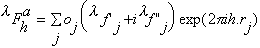
 ,
where oj is the occupancy of atom j, and
,
where oj is the occupancy of atom j, and
 and
and
 are the real and anomalous occupancies, respectively. If one sets both f' and
f" to an arbitrary value, the refinement of anomalous and dispersive occupancy
factors will adjust the relative values of
are the real and anomalous occupancies, respectively. If one sets both f' and
f" to an arbitrary value, the refinement of anomalous and dispersive occupancy
factors will adjust the relative values of
 .
Thus, it does not make a difference whether one inputs reasonable values for f'
and f", or if one inputs fake ones and lets the program refine occupancies.
However, I feel more comfortable with inputting reasonable values of the
anomalous scattering factors, because one gets occupancy values which "make
sense" : in this case, they should be the same for a given heavy atom position
throughout the data sets and then reflect the physical occupancy of the site.
In the other case, the occupancy will vary according to the values of
.
Thus, it does not make a difference whether one inputs reasonable values for f'
and f", or if one inputs fake ones and lets the program refine occupancies.
However, I feel more comfortable with inputting reasonable values of the
anomalous scattering factors, because one gets occupancy values which "make
sense" : in this case, they should be the same for a given heavy atom position
throughout the data sets and then reflect the physical occupancy of the site.
In the other case, the occupancy will vary according to the values of
 f' or f", and it should do so in a similar way for all sites at a
given wavelength. Therefore, the anomalous occupancy should be highest at the
maximum f" value, and the dispersive occupancy should be highest for the
difference between the minimum f' and the remote wavelength.
f' or f", and it should do so in a similar way for all sites at a
given wavelength. Therefore, the anomalous occupancy should be highest at the
maximum f" value, and the dispersive occupancy should be highest for the
difference between the minimum f' and the remote wavelength.
It is important to include as much data as possible in the phasing process. The
following criteria can be used to keep or select data :
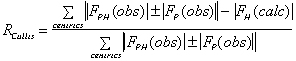 ;
;
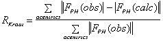 (isomorphous case)
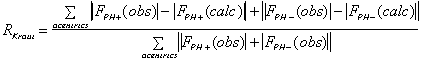 (anomalous case). R-Kraut should be as low as possible, and R-Cullis should
ideally be close to 0.5, and "typical" values are between 0.8 and 0.6.
(anomalous case). R-Kraut should be as low as possible, and R-Cullis should
ideally be close to 0.5, and "typical" values are between 0.8 and 0.6.
The figure of merit is the weighted mean of the cosine of the phase angle
deviation from  best. It is calculated as
 with
with
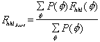 .
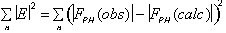
The phasing power is defined as
.
The phasing power is defined as
 with
with
 = rms lack of closure error. Both figure of merit and phasing power are plotted
as a function of resolution, and a given data set should ideally be cut-off at
a resolution where its phasing power drops below 1.
= rms lack of closure error. Both figure of merit and phasing power are plotted
as a function of resolution, and a given data set should ideally be cut-off at
a resolution where its phasing power drops below 1.
When the MAD phases are not sufficient to give an interpretable map, it is
straightforward to introduce other phasing information. A "native" data set
must be defined for all programs, except SHARP. All other data sets should be
scaled with respect to this native. Derivatives should be screened for phasing
power in order to keep only the useful data. Annex I shows an input and
excerpts of an output file from PHASES, illustrating the introduction of a
native, a mercury MAD data set and a single wavelength selenomethionine.
Several structures have been solved using a single heavy atom derivative
anomalous signal (e.g., Biou et al., 1995), and Eric de la Fortelle
showed that SHARP was quite able to solve structures this way. It takes cases
where a single heavy atom derivative (Pb in the mentioned case) gave a strong
anomalous signal. The phase ambiguity can then be resolved using solvent
flattening alone or solvent flattening and non crystallographic symmetry when
applicable. It is of course more difficult and more risky, but it may work when
one has no other choice.
You measure, process and scale data carefully on as good crystals as you can.
You try and minimize mosaic spread (work hard on cryoprotectants, use smaller
crystals).
All modern phasing methods work, it is more important to use one you're
familiar with, or you can get help with.
Then you can have an excellent experimental map to trace your chain
automatically, and excellent phases to refine your model against.
I apologise to all of the authors whose structures were omitted from the list
in Table 1. For lack of space I could not possibly include all of the relevant
references.
pdb entry - protein reference asymm. heavy atom res. (c) data used -
(a) unit (b) phasing method
content (d)
1CBP - blue copper (Guss et 10 kDa Cu 1 2.5Å MAD 4l- madsys
protein al., 1988)
? - streptavidin (Hendrickson 126 aa Se 2 3.1Å MAD 3l- madsys
et al.,
1989)
1RNH - RNase H (Yang et 156 aa Se 4 (6, 2.2Å MAD 3l- madsys
al., 1990) 13, 37, 36 (2.0)
/ 16)
1MSB - lectin domain (Weis et 110 aa Ho 4 2.5Å MAD 3l- madsys
from rat al., 1991)
mannose-binding
protein
1TEN - fibronectin (Leahy et 91 aa Se 1
(53, 3Å (1.8) MAD 4l- madsys
type III domain al., 1992) 39 / 21)
1ITH - homotetrameric (Kolatkar 2x141 aa Fe 1 5Å (2.5) MAD 4l + MIR -
hemoglobin et al., madsys
1992)
1HST - histone H5 (Ramakrishna 2x90 aa Se 2
(14, 2.6Å MAD 3l - mlphare
globular domain n et al., 15 / 21)
1993)
1HCN - HCG (Wu et al., 200 aa Se 4
(61, 2.6Å MAD 4l- madsys
1994) 55, 56, 80
/ 42)
1BGH - gene V protein (Skinner et 87 aa Se 1 (37/ 2.5Å MAD 3l - heavy
al., 1994) 21) & 2
1IRK - insulin (Hubbard et 306 aa Hg 2 2.5Å MAD 3l - madsys
receptor tyr kinase al., 1994) (2.1)
domain
1GPH - PRPP purine (Smith et 4x350 aa Fe 4 5 then MAD 3l - madsys
synthase al., 1994) 3Å
1OLA - OppA (Glover et 58.8 kDa U 8 2.3Å MAD 4l- mlphare
al., 1995)
1CNT - ciliary (McDonald 185 aa Yb 1 2.4Å MAD 4l- madsys
neutrophic factor et al.,
1995)
? - protein (Egloff et W + Hg 2.5Å MAD 3l + MIR +
phosphatase 1 al., 1995) 2-fold NCS-
phases
1ASU - avian sarcoma (Bujacz et 155 aa Se 4 (23, 2.2Å MAD 3l- phases
virus integrase al., 1995) 46, 41, 16 (1.7)
/ 33)
1TIG - IF3 C-terminal (Biou et 94 aa Se 2 (40, 2 Å MAD 3l - phases
domain al., 1995) 22 /20)
1GEO* - sulfite (Crane et 456 aa Fe 5 2.5Å MAD 3l + MIRAS
reductase al., 1995) (1.6) - madsys
1VHH - sonic hedgehog (Tanaka 200 aa Se 3 (19, 1.7Å MAD 4l - madlsq
N-terminal domain Hall et 43, 47/11)
al., 1995)
1IDO - integrin CR3 A (Lee et 192 aa Se 3 (17, 2Å (1.7) MAD 3l - mlphare
domain al., 1995) 17, 8/15)
1SVC - NFkB p50 (Müller et 364 aa + Se 5 (98, 3.4Å MAD 3l + MIR +
homodimer with DNA al., 1995) 19 bp 58, 49, (2.6) crystal
59, 66/ averaging -
70)+ I mlphare + madlsq
1NCG - cadherin (Shapiro et 110 aa Yb 1 2.1Å MAD 4l - madlsq
al., 1995)
? - mannose-binding (Burling et 230 aa Yb 1 1.8Å MAD 4l - xplor
protein al., 1996)
1RIE - rieske Fe-S (Iwata et 120 aa Fe 2 2.8Å MAD 3l - mlphare
protein fragment al., 1996) (1.5)
1TBG* - G protein (Sondek et 4x139 Gd 6 2.8Å MAD 3l - mlphare
ß dimer al., 1996) (2.1)
1FBT* - (Lee et 220 aa Se 4 2.8Å MAD 4l - mlphare
fructose-2,6-biphospha al., 1996) (2.5)
tase
1GSS - glutathione (Reinemer 2x211 aa Se 4 (16, 3Å (2.2) MAD 2l + MIR +
S-transferase et al., 22, 28, 22 2-fold NCS-
1996) / 26) + I mlphare
? - TFIIA/ TBP/ DNA (Geiger et 300 aa + Se / Br 5 3Å MAD 5l + MR -
complex al., 1996) 18 bpDNA mlphare
1WHI - ribosomal (Davies et 124 aa Se 2
dimer al., 1996) (2.1)
1FBT* - (Lee et 220 aa Se 4 2.8Å MAD 4l - mlphare
fructose-2,6-biphospha al., 1996) (2.5)
tase
1GSS - glutathione (Reinemer 2x211 aa Se 4 (16, 3Å (2.2) MAD 2l + MIR +
S-transferase et al., 22, 28, 22 2-fold NCS-
1996) / 26) + I mlphare
? - TFIIA/ TBP/ DNA (Geiger et 300 aa + Se / Br 5 3Å MAD 5l + MR -
complex al., 1996) 18 bpDNA mlphare
1WHI - ribosomal (Davies et 124 aa Se 2
(32, 2 Å MAD 3l + MIR -
protein L14 al., 1996) 21 / 14) (1.5) phases
1DKX - DnaK chaperone (Zhu et 218 + 7aa Se 6 2.3Å MAD 4l - madsys
+ peptide al., 1996)
1UMU - UmuD' protein (Peat et 2x116 aa Se 4 (26, 2.5Å MAD 4l - madsys
al., 1996) 48, 25, 31 + multan
/ 24)
1TEN - fibronectin (Leahy et 90 aa Se 1 (53 / 1.8Å MAD 4l - madsys
type III repeat al., 1996) )
1ZEN - class II (Cooper et 39 kDa Se 6 (15, 2.5Å MAD 3l + MIR -
aldolase al., 1996) 33, 26, mlphare
31, 44,
23/ 36)
Table II Non exhaustive list of MAD structures to date.
(a) Pdb entry code followed by *: coordinates release still pending at time of
writing. When replaced with ? : entry not found in pdb; (b) heavy atom : type,
number and temperature factors (Å2) of the corresponding SD or
SE atoms in the released pdb entry for selenomethionine protein, followed with
the mean overall temperature factor. (c) second figure between parentheses
gives resolution used for refinement when different from the MAD experiment
resolution.
(d) References for phasing programs : Heavy (Terwillinger, 1994a &b),
Mlphare (Otwinowski, 1991), Madsys (Hendrickson et al., 1988;
Hendrickson, 1991), Phases (Furey and Swaminathan, 1997), Xplor version 3.8x
(Burling et al., 1996).
Bertrand, J.A., Auger, G., Fanchon, E., Martin, L., Blanot, D., van Heijenoort,
J. and Dideberg, O. (1997) crystal structure of
UDP-N-acetylmuramoyl-L-alanine:D-glutamata ligase from Escherichia
coli. EMBO J., (In Press)
Biou, V., Shu, F. and Ramakrishnan, V. (1995) X-ray crystallography shows that
translational initiation factor IF3 consists of two compact alpha/beta domains
linked by an alpha-helix. EMBO J., 14, 4056-4064.
Bujacz, G., Jaskolski, M., Alexandratos, J., Wlodawer, A., Merkel, G., Katz,
R.A. and Skalka, A.M. (1995) High-resolution structure of the catalytic domain
of avian sarcoma virus integrase. J.Mol.Biol., 253, 333-346.
Burling, F.T., Weis, W.I., Flaherty, K.M. and Brunger, A.T. (1996) Direct
observation of protein solvation and discrete disorder with experimental
crystallographic phases. Science, 271, 72-77.
Cooper, S.J., Leonard, G.A., McSweeny, S.M., Thompson, A.M., Naismith, J.H.,
Qamar, S., Plater, A., Berry, A. and Hunter, W.N. (1996) The crystal structure
of a class II fructose-1,6-biphosphate aldolase shows a novel binuclear
metal-binding active site embedded in a familiar fold. Structure,
4, 1303-1315.
Crane, B.R., Siegel, L.M. and Getzoff, E.D. (1995) Sulfite reductase structure
at 1.6 A: evolution and catalysis for reduction of inorganic anions.
Science, 270, 59-67.
Cusack, S. , 1996. (UnPub)
Davies, C., White, S.W. and Ramakrishnan, V. (1996) The crystal structure of
ribosomal protein L14 revels an important organisational component of the
translational apparatus. Structure, 4, 55-65.
de la Fortelle, E. and Bricogne, G. (1997) Maximum likelihood heavy-atom
parameter refinement for multiple isomorphous replacement and multivavelength
anomalous diffraction methods. In Carter, C.W. and Sweet, R.M. (ed.)Methods
in Enzymology vol 276, Academic Press, Orlando, Fl: pp. 472-494.
Egloff, M.P., Cohen, P.T., Reinemer, P. and Barford, D. (1995) Crystal
structure of the catalytic subunit of human protein phosphatase 1 and its
complex with tungstate. J.Mol.Biol., 254, 942-959.
Furey, W. and Swaminathan, S. (1997) Phases-95 : a program package for the
processing and analysis of diffraction data from macromolecules. In Carter, C.
and Sweet, R.M. (ed.)Methods in Enzymology, Academic Press, Orlando, Fl:
Geiger, J.H., Hahn, S., Lee, S. and Sigler, P.B. (1996) Crystal structure of
the yeast TFIIA/TBP/DNA complex . Science, 272, 830-836.
Glover, I.D., Denny, R.C., Nguti, N.D., McSweeny, S.M., Kinder, S.H., Thompson,
A.M., Dodson, E.J., Wilkinson, A.J. and Tame, J.R. (1995) Structure
determination of OppA at 2.3Å resolution using multiple-wavelength
anomalous dispersion methods. Acta Cryst., D51, 39-47.
Guss, J.M., Merritt, E.A., Phizackerley, R.P., Hedman, B., Murata, M., Hodgson,
K.O. and Freeman, H.C. (1988) Phase determination by Multiple wavelength X-ray
diffraction : crystal structure of a basic "blue" copper protein from
cucumbers. Science, 241, 806-811.
Hendrickson, W.A., Pähler, A., Smith, J.L., Satow, Y., Merritt, E.A. and
Phizackerley, R.P. (1989) Crystal structure of core streptavidin determined
from multiwavelength anomalous diffraction of synchrotron radiation.
Proc.Natl.Acad.Sci.U.S.A., 86, 2190-2194.
Hendrickson, W.A. (1991) Determination of macromolecular structures from
anomalous diffraction of synchrotron radiation. Science, 254,
51-58.
Hendrickson, W.A.H., Smith, J.L., Phizackerley, R.P. and Merritt, E.A. (1988)
Crystallographic structure analysis of lamprey hemoglobin from anomalous
dispersion of synchrotron radiation. Proteins, 4, 77.
Hubbard, S.R., Wei, L., Ellis, L. and Hendrickson, W.A. (1994) Crystal
structure of the tyrosine kinase domain of the human insulin receptor .
Nature, 372, 746-754.
Iwata, S., Saynovits, M., Link, T.A. and Michel, H. (1996) Structure of a water
soluble fragment of the 'Rieske' iron-sulfur protein of the bovine heart
mitochondrial cytochrome bc1 complex determined by MAD phasing at 1.5Å
resolution. Structure, 4, 5678-579.
Karle, J. (1980) Some developments in anomalous dispersion for the structural
investigation of macromolecular systems in biology. Int.J.Quant.Chem.,
7, 357-367.
Kolatkar, P.R., Ernst, S.R., Hackert, M.L., Ogata, C.M., Hendrickson, W.A.,
Merritt, E.A. and Phizackerley, R.P. (1992) Structure determination and
refinement of homotetrameric hemoglobin from Urechis caupo at 2.5 A resolution.
Acta Crystallogr.B, 48, 191-199.
Leahy, D.J., Hendrickson, W.A., Aukhil, I. and Erickson, H.P. (1992) Structure
of a fibronectin type III domain from tenascin phased by MAD analysis of the
selenomethionyl protein. Science, 258, 987-991.
Leahy, D.J., Hendrickson, W.A., Aukhil, I. and Erickson, H.P. (1996) Structure
of a fibronectin type III domain from tenascin phased by MAD analysis of the
selenomethionyl protein. Science, 258, 987-991.
Lee, J.O., Rieu, P., Arnaout, M.A. and Liddington, R. (1995) Crystal structure
of the A domain from the alpha subunit of integrin CR3 (CD11b/CD18).
Cell, 80, 631-638.
Lee, Y.H., Ogata, C., Pflugrath, J.W., Levitt, D.G., Sarma, R., Banaszak, L.J.
and Pilkis, S.J. (1996) Crystal structure of the rat liver
fructose-2,6-bisphosphatase based on selenomethionine multiwavelength anomalous
dispersion phases. Biochemistry, 35, 6010-6019.
Leslie, A.G.W. Program ipmosflm version 5.4, 1996. (UnPub)
McDonald, N.Q., Panayotatos, N. and Hendrickson, W.A. (1995) Crystal structure
of dimeric human ciliary neurotrophic factor determined by MAD phasing. EMBO
J., 14, 2689-2699.
Müller, C.W., Rey, F.A., Sodeka, M., Verdine, G.L. and Harrison, S.C.
(1995) Structure of the NF-Kappa B P50 homodimer bound to DNA. Nature,
373, 311-317.
Otwinowski, Z. (1991) . In Wolf, W., Evans, P.R. and Leslie, A.G.W.
(ed.)Isomorphous replacement and anomalous scattering, Daresbury
Laboratory, Warrington: pp. 80.
Peat, T.S., Frank, E.G., McDonald, J.P., Levine, A.S., Woodgate, R. and
Hendrickson, W.A. (1996) structure of the UMUD' protein and its regulation in
response to DNA damage . Nature,
380, 727.
Ramakrishnan, V., Finch, J.T., Graziano, V., Lee, P.L. and Sweet, R.M. (1993)
Crystal structure of globular domain of histone H5 and its implications for
nucleosome binding. Nature, 362, 219-223.
Ramakrishnan, V. and Biou, V. (1997) Treatment of MAD as a special case of MIR.
In Carter, C. and Sweet, R.M. (ed.)Methods in Enzymology vol 276,
Academic Press, Orlando, Fl: pp. 538-557.
Reid, R.J. (1996) As MAD as can be. Structure, 4, 11-14.
Reinemer, P., Prade, L., Hof, P., Neuefeind, T., Huber, R., Zettl, R., Palme,
K., Schell, J., Koelln, I., Bartunik, H.D. and Bieseler, B. (1996)
Three-dimensional structure of glutathione S-transferase from Arabidopsis
thaliana at 2.2 A resolution: structural characterization of
herbicide-conjugating plant glutathione S-transferases and a novel active site
architecture. J.Mol.Biol., 255, 289-309.
Shapiro, L., Fannon, A.M., Kwong, P.D., Thompson, A.M., Lehman, M.S., Grubel,
G., Legrand, J.-F., Als-Nielsen, J., Colman, D.R. and Hendrickson, W.A. (1995)
structural basis of cell-cell adhesion by cadherins. Nature, 374,
327.
Skinner, M.M., Zhang, H., Leschnitzer, D.H., Guan, Y., Bellamy, H., Sweet,
R.M., Gray, C.W., Konings, R.N., Wang, A.H. and Terwilliger, T.C. (1994)
Structure of the gene V protein of bacteriophage f1 determined by
multiwavelength x-ray diffraction on the selenomethionyl protein.
Proc.Natl.Acad.Sci.U.S.A., 91, 2071-2075.
Smith, J.L., Zaluzec, E.J., Wery, J.P., Niu, L., Switzer, R.L., Zalkin, H. and
Satow, Y. (1994) Structure of the allosteric regulatory enzyme of purine
biosynthesis. Science, 264, 1427-1433.
Sondek, J., Bohm, A., Lambright, D.G., Hamm, H.E. and Sigler, P.B. (1996)
Crystal structure of a GA protein beta gamma dimer at 2.1A resolution.
Nature, 379, 369-374.
Tanaka Hall, T.M., Porter, J.A., Beachy, P.A. and Leahy, D.J (1995) A potential
catalytic site revealed by the 1.7Å crystal structure of the
amino-terminal signalling domain of Sonic hedgehog. Nature, 378,
212-216.
Terwillinger, T.C. (1994a) MAD phasing : treatment of dispersive differences as
isomorphous replacement information. Acta Crystallogr.D, D50,
17-23.
Terwillinger, T.C. (1994b) MAD phasing : Bayesian estimates of FA. Acta
Crystallogr.D, D50, 11-16.
Weis, W.I., Kahn, R., Fourme, R., Drickamer, K. and Hendrickson, W.A. (1991)
Structure of the calcium-dependent lectin domain from a rat mannose-binding
protein determined by MAD phasing. Science, 254, 1608-1615.
Wu, H., Lustbader, J.W., Liu, Y., Canfield, R.E. and Hendrickson, W.A. (1994)
Structure of human chorionic gonadotropin at 2.6Å resolution from MAD
analysis of the selenomethionyl protein. Structure, 2, 545-558.
Wu, H. and Hendrickson, W.A. (1996) The analytical approach of phasing by
multiwavelength anomalous dispersion. IUCR abstracts, C55.(Abstract)
Yang, W., Hendrickson, W.A., Crouch, R.J. and Satow, Y. (1990) Structure of
ribonuclease H phased at 2 A resolution by MAD analysis of the selenomethionyl
protein. Science, 249, 1398-1405.
Zhu, X., Zhao, X., Burkholder, W.F., Gragerov, A., Ogata, C.M., Gottesman, M.E.
and Hendrickson, W.A. (1996) Structural analysis of substrate binding by the
molecular chaperone DnaK. Science, 272, 1606-1614.
NOTE from CCP4 : this data has not converted correctly
to html and as yet should not be used. This is not a problem with the
origional data submited by the author
Example for an input file to PHASES where the MAD data has been scaled to a
native data set, and an additional mercury derivative collected elsewhere with
a higher occupancy was also used.
hgmad.pam
0 4
29.564100 18.059999 12.837400 6.899120
1.211520 7.056390 .284738 20.748199 12.608900
-14.40000 10.50000
29.564100 18.059999 12.837400 6.899120
1.211520 7.056390 .284738 20.748199 12.608900
-23.00000 7.00000
29.564100 18.059999 12.837400 6.899120
1.211520 7.056390 .284738 20.748199 12.608900
-10.87000 9.88000
29.564100 18.059999 12.837400 6.899120
1.211520 7.056390 .284738 20.748199 10.626800
-4.99000 7.68600
6 1 1
hgmad5.hkl
hgmad l1 anomalous
natl1_ano.hkl
4.00 5.00 2 .9957 .0 2.9489 .5462E-01 -.1775E+03 .1063E+07
.5844E+06
2
Hg -.11140 -.18788 -.08980 20.00000 1.51119 21
Hg -.36478 -.16421 -.52978 20.00000 1.20566 21
hgmad l2 anomalous
natl2_ano.hkl
4.00 5.00 2 1.0027 .0 2.2748 .6032E-01 -.2386E+03 .1642E+07
.1047E+07
2
Hg -.11616 -.18952 -.09076 20.00000 1.43557 22
Hg -.36362 -.16569 -.52917 20.00000 1.12660 22
madc l1 isomorphous
natl1_iso.hkl
4.00 5.00 0 1.0046 .0 4.3930 .7547E-01 -.1094E+03 .1181E+07
.9751E+06
2
Hg -.11017 -.18803 -.09007 20.00000 1.23379 21
Hg -.36553 -.16387 -.53047 20.00000 1.00647 21
madc l2 isomorphous
natl2_iso.hkl
4.00 5.00 0 1.0000 .0 4.6351 .5751E-01 .1684E+03 .7555E+06
.1108E+07
2
Hg -.10891 -.18749 -.08981 20.00000 1.20896 22
Hg -.36537 -.16366 -.53040 20.00000 1.00433 22
madc l3 isomorphous
natl3_iso.hkl
4.00 5.00 0 1.0000 .0 4.0734 .5735E-01 .2727E+03 .5969E+06
.1344E+07
2
Hg -.10885 -.18771 -.08972 20.00000 1.22450 23
Hg -.36536 -.16375 -.53036 20.00000 1.00473 23
madc hg hamburg isomorphous
nathgderiv_iso.hkl
4.00 5.00 0 1.0000 .0 6.9056 .7391E-01 -.1897E+03 .7521E+07
.6809E+07
2
Hg -.11096 -.18758 -.08918 20.00000 1.18599 24
Hg -.36646 -.16443 -.52977 20.00000 .96625 24
2 .20 18 0 1 0 1
1 SET 1
0 0 0 1 0
0 0 0 0 0
0 0 1
2 SET 2
0 0 0 1 0
0 0 0 0 0
0 0 1
......etc.
Excerpts from the PHASIT log file from the above input file.
The breakdown of phasing power vs resolution is given only for one dataset.
STATISTICS FOR SET 1 AFTER REFINEMENT
R KRAUT = .045 FOR 12662 ACENTRIC REFLECTIONS
STATISTICS FOR SET 2 AFTER REFINEMENT
R KRAUT = .056 FOR 10920 ACENTRIC REFLECTIONS
STATISTICS FOR SET 3 AFTER REFINEMENT
R CULLIS = .558 FOR 319 CENTRIC REFLECTIONS
R KRAUT = .038 FOR 3764 ACENTRIC REFLECTIONS
STATISTICS FOR SET 4 AFTER REFINEMENT
R CULLIS = .620 FOR 834 CENTRIC REFLECTIONS
R KRAUT = .045 FOR 5958 ACENTRIC REFLECTIONS
STATISTICS FOR SET 5 AFTER REFINEMENT
R CULLIS = .623 FOR 770 CENTRIC REFLECTIONS
R KRAUT = .049 FOR 5793 ACENTRIC REFLECTIONS
STATISTICS FOR SET 6 AFTER REFINEMENT
R CULLIS = .513 FOR 648 CENTRIC REFLECTIONS
R KRAUT = .110 FOR 5315 ACENTRIC REFLECTIONS
--------------- START OF NEXT PHASING CYCLE ---------------
INDIVIDUAL DATA SET RESULTS BASED ON UPDATED HEAVY ATOM AND E VALUES
SET 1 madhg l1 anomalous
MEAN FIGURE OF MERIT = .389 FOR 6331 REFLECTIONS
SET 2 madhg l2 anomalous
MEAN FIGURE OF MERIT = .148 FOR 5460 REFLECTIONS
SET 3 madc l1 isomorphous
MEAN FIGURE OF MERIT = .508 FOR 4083 REFLECTIONS
MEAN FIGURE OF MERIT = .733 FOR 319 CENTRIC REFLECTIONS
MEAN FIGURE OF MERIT = .488 FOR 3764 ACENTRIC REFLECTIONS
SET 4 madc l2 isomorphous
MEAN FIGURE OF MERIT = .474 FOR 6792 REFLECTIONS
MEAN FIGURE OF MERIT = .677 FOR 834 CENTRIC REFLECTIONS
MEAN FIGURE OF MERIT = .446 FOR 5958 ACENTRIC REFLECTIONS
SET 5 madc l3 isomorphous
MEAN FIGURE OF MERIT = .468 FOR 6563 REFLECTIONS
MEAN FIGURE OF MERIT = .654 FOR 770 CENTRIC REFLECTIONS
MEAN FIGURE OF MERIT = .443 FOR 5793 ACENTRIC REFLECTIONS
SET 6 madc hg hamburg isomorphous
MEAN FIGURE OF MERIT = .396 FOR 5963 REFLECTIONS
MEAN FIGURE OF MERIT = .569 FOR 648 CENTRIC REFLECTIONS
MEAN FIGURE OF MERIT = .375 FOR 5315 ACENTRIC REFLECTIONS
********** RESULTS FROM COMBINED PROBABILITY DISTRIBUTIONS **********
ACENTRIC REFLECTIONS INCLUDED IF 1 OR MORE DATA SETS CONTRIBUTED IN PHASE
CALCULATION
MEAN FIGURE OF MERIT = .716 FOR 7538 PHASED REFLECTIONS
MEAN PHASE SHIFT FROM PREVIOUS CYCLE = 1.22 DEGREES
MEAN FIGURES OF MERIT AS FUNCTION OF FP MAGNITUDE
MEAN FOM = .585 MEAN FP = 1558.76 NUM REFL = 753
MEAN FOM = .702 MEAN FP = 2395.57 NUM REFL = 753
MEAN FOM = .747 MEAN FP = 3105.68 NUM REFL = 753
MEAN FOM = .731 MEAN FP = 3784.38 NUM REFL = 753
MEAN FOM = .752 MEAN FP = 4456.45 NUM REFL = 753
MEAN FOM = .744 MEAN FP = 5162.72 NUM REFL = 753
MEAN FOM = .735 MEAN FP = 6018.64 NUM REFL = 753
MEAN FOM = .723 MEAN FP = 7012.22 NUM REFL = 753
MEAN FOM = .732 MEAN FP = 8504.27 NUM REFL = 753
MEAN FOM = .708 MEAN FP = 11671.32 NUM REFL = 753
MEAN FIGURES OF MERIT AS FUNCTION OF RESOLUTION
MEAN FOM = .723 MEAN D = 4.07 NUM REFL = 753
MEAN FOM = .694 MEAN D = 4.24 NUM REFL = 753
MEAN FOM = .699 MEAN D = 4.42 NUM REFL = 753
MEAN FOM = .705 MEAN D = 4.64 NUM REFL = 753
MEAN FOM = .705 MEAN D = 4.90 NUM REFL = 753
MEAN FOM = .718 MEAN D = 5.24 NUM REFL = 753
MEAN FOM = .716 MEAN D = 5.71 NUM REFL = 753
MEAN FOM = .714 MEAN D = 6.40 NUM REFL = 753
MEAN FOM = .750 MEAN D = 7.60 NUM REFL = 753
MEAN FOM = .734 MEAN D = 11.87 NUM REFL = 753
PHASING POWER BREAKDOWN BASED ON CURRENT PROTEIN PHASES
SET 1 madhg l1 anomalous
MEAN D = 8.63 PHASING POWER = 2.00 MEAN BIAS = 91.4 REFL=
633
MEAN D = 6.20 PHASING POWER = 2.93 MEAN BIAS = 91.9 REFL=
633
MEAN D = 5.52 PHASING POWER = 3.06 MEAN BIAS = 86.9 REFL=
633
MEAN D = 5.13 PHASING POWER = 2.64 MEAN BIAS = 88.6 REFL=
633
MEAN D = 4.85 PHASING POWER = 2.38 MEAN BIAS = 85.7 REFL=
633
MEAN D = 4.63 PHASING POWER = 2.06 MEAN BIAS = 93.8 REFL=
633
MEAN D = 4.45 PHASING POWER = 2.24 MEAN BIAS = 89.6 REFL=
633
MEAN D = 4.30 PHASING POWER = 2.06 MEAN BIAS = 91.4 REFL=
633
MEAN D = 4.17 PHASING POWER = 2.15 MEAN BIAS = 93.6 REFL=
633
MEAN D = 4.05 PHASING POWER = 1.86 MEAN BIAS = 93.3 REFL=
633
MEAN D = 4.00 PHASING POWER = .98 MEAN BIAS = 62.0 REFL=
1
OVERALL MEAN D= 5.19 PHASING POWER = 2.29 M.R.E. = .73 MEAN BIAS =
90.6 REFL= 6331
UPDATED E VALUES BASED ON NEW PROTEIN PHASES
NRFL <F> RMS E E FIT DEL E
316 1433.3 586459.1 953553.1 -367094.1
316 1927.6 1238142.4 915128.3 323014.1
316 2296.8 700552.8 905066.5 -204513.8
316 2650.5 744915.5 910378.9 -165463.4
316 2940.9 920513.4 925675.9 -5162.6
316 3221.9 1935495.5 949859.1 985636.4
316 3504.3 912075.1 983473.8 -71398.6
316 3803.2 904681.1 1029200.4 -124519.3
316 4102.3 1017892.9 1085436.8 -67543.9
316 4436.8 1125683.5 1160689.8 -35006.3
316 4739.0 1246982.5 1239951.1 7031.4
316 5026.7 1377596.4 1325317.4 52279.0
316 5372.2 1303630.9 1440618.3 -136987.4
316 5731.4 1461523.4 1575311.5 -113788.1
316 6210.0 1776409.8 1778172.0 -1762.3
316 6661.4 1947772.3 1994115.0 -46342.8
316 7304.2 2016219.8 2342693.0 -326473.3
316 8054.2 2656859.8 2810452.8 -153593.0
316 9120.4 4160179.3 3588630.8 571548.5
316 11456.4 5638618.0 5758275.0 -119657.0
(...)
SET 3 madc l1 isomorphous
OVERALL MEAN D= 5.59 PHASING POWER = 3.20 M.R.E. = .52 MEAN BIAS =
87.7 REFL= 4083
UPDATED E VALUES BASED ON NEW PROTEIN PHASES
SET 4 madc l2 isomorphous
OVERALL MEAN D= 5.68 PHASING POWER = 2.36 M.R.E. = .53 MEAN BIAS = 88.3
REFL= 6792
SET 5 madc l3 isomorphous
OVERALL MEAN D= 5.69 PHASING POWER = 2.35 M.R.E. = .51 MEAN BIAS =
88.0 REFL= 6563
SET 6 madc hg hamburg isomorphous
OVERALL MEAN D= 6.12 PHASING POWER = 1.63 M.R.E. = .64 MEAN BIAS =
84.6 REFL= 5963