Case
Study: MAD phasing of desulphoredoxin, an Fe metalloprotein.
Ian D. Glover and Don Nguti.
Physics Department, Keele University, Keele, Staffs. ST5 5BG.
Introduction.
Desulphoredoxin is a small iron containing metalloprotein, consisting of a
dimer of 36 residue chains each coordinating an iron atom. Data collected about
the Fe absorbtion edge of 1.74Å , wavelengths being set with reference to XANES
spectra recorded from a single crystal, were used to determine the positions of
the anomalously scattering Fe atom and hence, using MLPHARE calculate an
electron density map.
Desulphoredoxin is an Fe-S protein isolated from Desulphovibrio
gigas,(Mouri et al., 1977, Bruschi et al., 1979) comprised of
two 36 residue monomers, each coordinating an iron atom, which form a dimers
with an Mr of 7740. Each of the monomers has four Cys residues expected to
coordinate the iron atom. Most biochemical and spectroscopic evidence points to
a similar coordination of iron but in relation to rubredoxin, higher symmetry
in Fe binding is anticipated.
Good quality crystals of desulphoredoxin were first reported in 1980 (Seiker et
al., 1980), but no suitable derivatives have been prepared. As a small
metalloprotein it presented a good case for structure determination using MAD
methods. With two Fe atoms in a small protein significant anomalous scattering
contributions are expected, the maximal anomalous diffraction ratios
(Hendrickson, 1991) of 5% and 4.8% for the absorptive and dispersive
contributions respectively.
Data Collection.
Desulphoredoxin crystallises in space group P3121 (or its enantiomer) with cell
dimensions a = b = 42.28Å , c = 72.46Å , and  =
120o. The crystals grow to
approximately 0.3mm in the largest dimensions and are relatively radiation
stable. All data were collected on station 9.5(Thompson et al., 1992) at
the Daresbury SRS using an 18cm diameter MAR image plate detector and a channel
cut Si(111) double crystal monochromator. MAD data were collected at four
wavelengths, three close to the Fe-K edge, determined from XANES scans from a
crystal and a fourth, higher resolution, dataset recorded at a remote
wavelength. As the data were collected at room temperature all measurements
contributing to a particular phase determination were collected as close
together in time as possible. Initial calibration of the incident X-ray
wavelengths was performed using the iron edge in a piece of magnetic tape, and
thereafter x-ray wavelengths calculated using the monochromator angle. Due to
the goniometer geometry the closest possible approach of the detector limited
data collected at the longer wavelengths to approximately 3Å resolution.
=
120o. The crystals grow to
approximately 0.3mm in the largest dimensions and are relatively radiation
stable. All data were collected on station 9.5(Thompson et al., 1992) at
the Daresbury SRS using an 18cm diameter MAR image plate detector and a channel
cut Si(111) double crystal monochromator. MAD data were collected at four
wavelengths, three close to the Fe-K edge, determined from XANES scans from a
crystal and a fourth, higher resolution, dataset recorded at a remote
wavelength. As the data were collected at room temperature all measurements
contributing to a particular phase determination were collected as close
together in time as possible. Initial calibration of the incident X-ray
wavelengths was performed using the iron edge in a piece of magnetic tape, and
thereafter x-ray wavelengths calculated using the monochromator angle. Due to
the goniometer geometry the closest possible approach of the detector limited
data collected at the longer wavelengths to approximately 3Å resolution.
Wavelength selection
The XANES spectrum were recorded from a single crystal of desulphoredoxin is
shown in figure 1. The spectrum was transformed using the Kramers-Kronig
(Kronig & Kramers, 1928) transform, to obtain experimental values of f' and
f" (table 1). The values of the anomalous scattering coefficients were used to
select the nominal wavelengths,  1 at 1.744Å
, the first point of inflection on
the f" curve, and therefore the minimum or most negative value on the f' curve.
The second wavelength, 2 was selected at 1.740Å
, the maximum on the f" curve,
this data set will yield the greatest Bijvoet or Friedel differences. The third
wavelength, 3, was selected at 1.7285Å
, remote from the edge. The fourth
wavelength was collected at 0.9Å , where the incident flux on station 9.5 is
significantly higher and with the same data collection geometry allowed much
higher resolution data (1.8Å ) to be collected. During data collection at the
longer wavelengths the monochromator second crystal was detuned to avoid
harmonic contamination of the incident beam.
1 at 1.744Å
, the first point of inflection on
the f" curve, and therefore the minimum or most negative value on the f' curve.
The second wavelength, 2 was selected at 1.740Å
, the maximum on the f" curve,
this data set will yield the greatest Bijvoet or Friedel differences. The third
wavelength, 3, was selected at 1.7285Å
, remote from the edge. The fourth
wavelength was collected at 0.9Å , where the incident flux on station 9.5 is
significantly higher and with the same data collection geometry allowed much
higher resolution data (1.8Å ) to be collected. During data collection at the
longer wavelengths the monochromator second crystal was detuned to avoid
harmonic contamination of the incident beam.
   Dataset      Wavelength (Å)       f'             f''
      1             1.7444         -8.091         1.993
      2             1.7405         -6.096         4.337
      3             1.7284         -4.054         3.975
      4             0.9000         -1.100         2.900
Table 1. The anomalous scattering factors for iron in desulphoredoxin
at the wavelengths selected for data collection, the first three are derived
from the Kramers-Kronig transform of the recorded XANES spectrum shown in
figure 1.
One crystal was used in the collection of the three near edge data sets,
1, 2
and 3,
and a second crystal used to record the fourth, 0.9Å wavelength,
4
data set. The crystals were accurately aligned with the c* axis parallel to the
spindle axis. In this orientation there were no mirror related reflection
recorded on the same image, all mirror related reflections were recorded by
inverting the crystal, i.e. recording data at  and + 1800. A total of 940 (
 = 3 or 40) of data were collected at wavelengths 1,2, and 3 and 700 (
= 2o) at
the fourth wavelength
= 3 or 40) of data were collected at wavelengths 1,2, and 3 and 700 (
= 2o) at
the fourth wavelength
Scaling and merging of the data.
Initial data reduction was carried out using the MOSFLM (Leslie, 1992) suite of
programs after the determination of the initial orientation matrix using REFIX.
Regardless of the phasing approach to be used, MADSYS or MLPHARE, once
collected the data must be scaled, both within datasets and for the MAD
analysis, between datasets to reduce differences due to crystal decay,
absorbtion and any variation in detector response. Scale factors were
calculated initially using ROTAVATA (CCP4, 1994) which calculated a single
scale factor (Fox & Holmes, 1966) that is applied to all reflections in a
particular batch, usually a single image. This means that symmetry related
reflection falling on consecutive batches can have very different scale
factors. Since the scaling is based on all symmetry related reflections within
a dataset whose intensities are expected to be equal a continuously varying
scale factor may be more appropriate, such as the approach used in SCALA (P.R.
Evans, this volume) where the scale factor is a continuous function of rotation
angle and detector position.
1) ROTAVATA
Scale and temperature factors between batches within each dataset were
initially calculated using ROTAVATA and applied using AGROVATA. The results are
set out in detail in tables 2 and 3. Taking the three datasets collected at
wavelengths close to the iron edge, the overall RSYMM values are 14.6%, 15.2%
and 13.8% respectively for the 1,
2 and
3 datasests which compare very
unfavourably with the dataset recorded at 0.9Å wavelength. This poor scaling is
clearly seen in the tables of batch scale and temperature factors calculated
by ROTAVATA which show a large variation in scale factors and very significant
variation in temperature factors. This poor scaling contributes to the mediocre
quality of the merged data. Few batches had low RSYMM values and the signal to
noise, as judged by the value of I/ (I) was poor, averaging 3.5. Contrasting
with this is the 4 dataset where
the scale factors follow a regular
progression, the biggest variations occurring either side of a beam refill and
the temperature factors vary only slightly. The RSYMM values are significantly
lower and the signal to noise better with an average I/(I) of 17.5.
(I) was poor, averaging 3.5. Contrasting
with this is the 4 dataset where
the scale factors follow a regular
progression, the biggest variations occurring either side of a beam refill and
the temperature factors vary only slightly. The RSYMM values are significantly
lower and the signal to noise better with an average I/(I) of 17.5.
This variation is seen despite the fact that the data were collected from
similar sized crystals of the same shape. Furthermore it should be noted that
the RSYMM value of the 4
data at 3.05Å resolution is only 1.8%. The only
difference between the data is that the 1,
2 and 3
data were collected at
longer wavelengths and that higher absorbtion at these wavelengths is having a
significant effect on the internal consistency. Data of this quality is clearly
going to present problems for the subsequent MAD analysis when the expected
values for the largest anomalous and dispersive diffraction ratios are 5% and
4.8% respectively.
 Dataset     Wavelength (Å)     IMEAN/       RSYMM        Nobs
   1          1.7444            3.54        0.146       6857
   2          1.7405            3.29        0.152       6889
   3          1.7284            3.95        0.138       6766
   4          0.9000           17.46        0.034      20308
Table 2. Summary of the overall batch symmetry R-factors for the four
MAD datasets. Note that the fourth wavelength extends to 1.8Å resolution.
                      DATASET 1                  DATASET  4
   BATCH         SCALE           B           SCALE           B
     1           1.000          0.0          1.000          0.0
     2           1.445          5.0          0.965          -0.2
     3           1.970          -0.7         1.007          -0.1
     4           1.499          6.0          0.937          -0.6
     5           1.957          7.9          0.951          -0.6
     6           2.345          -2.9         0.988          -0.7
     7           2.520          3.6          0.992          -0.8
     8           2.201          1.4          1.032          -0.8
     9           2.505          0.3          1.060          -0.8
     10          2.113          4.6          1.114          -0.9
     11          2.827          5.0          1.077          -0.9
     12          3.504          4.0          1.099          -1.0
     13          2.134          4.4          1.092          -1.1
     14          2.574          5.7          1.156          -1.4
     15          2.833          6.5          1.185          -0.7
     16          2.883          4.3          1.235          -1.0
     17          2.925          4.1          1.222          -1.3
     18          3.081          3.3          1.263          -1.1
     19          3.193          1.1          1.248          -1.3
     20          3.385          -0.6         1.268          -1.2
     21          3.758          0.3          1.298          -1.4
     22          4.021          -1.2         1.305          -1.4
     23          4.434          -2.6         1.412          -1.5
     24          4.811          -4.1         1.380          -1.5
     25          2.453          -2.8         1.404          -1.6
     26          2.918          -2.6         1.423          -1.4
     27          3.153          3.6          1.445          -1.9
     28                                      1.053          -1.6
     29                                      1.061          -1.6
     30                                      1.069          -2.2
     31                                      1.066          -2.0
     32                                      1.082          -2.3
     33                                      1.076          -2.2
     34                                      1.073          -2.3
     35                                      1.089          -2.2
Table 3. a)The scale and temperature factor (B) for the
datasets 1 and 4,
recorded at 1.7444Å and 0.900Å wavelengths calculated using
the program ROTAVATA. The abrupt change in scale factors in the short
wavelength data at batch 28 is due to a beam refill. b) Values for the
1 dataset after scaling using SCALA.
   BATCH         SCALE           B
     1           0.279          0.0
     2           0.334         -0.47
     3           0.416         -1.16
     4           0.534         -3.72
     5           0.333         -1.95
     6           0.414         -1.45
     7           0.594         -3.298
     8           0.5624        -4.62
     9           0.652         -5.37
     10          0.504         -2.65
     11          0.657         -2.87
     12          0.878         -2.61
     13          0.535         -1.61
     14          0.583         -2.30
     15          0.644         -2.87
     16          0.705         -2.32
     17          0.711         -3.09
     18          0.771         -4.31
     19          0.872         -4.69
     20          0.970         -5.93
     21          1.014         -7.12
     22          1.149         -7.91
     23          1.334         -9.61
     24          1.506         -11.00
     25          0.7614        -8.83
     26          0.873         -10.21
     27          0.940         -10.68
2) SCALA.
The program SCALA was used to calculate scale and temperature factors for each
dataset prior to merging in AGROVATA. SCALA differs in methodology in that it
calculates a three dimensional scale factor for each reflection taking into
account rotation angle and its position on the detector. This methodology has
significant benefits when applied to this case where sample absorbtion is
anticipated to have a large effect on the internal consistency of the data. The
results from scaling and merging with SCALA/AGROVATA (tables 3 and 4) show a
very significant improvement for the data collected at long wavelengths. The
signal to noise ratios have increased considerably and the consistency,
typically from approx 12% to 3%. The short wavelength data, however, shows very
little improvement.
Table 4. a) Summary of the overall batch symmetry R-factors for the
four MAD datasets scaled using SCALA (data compared to 3.05Å resolution) and b)
the merging statistics and multiplicity (Mult.) from AGROVATA.
a)
 Dataset      Wavelength (Å)      IMEAN/         R           Nobs
   1             1.7444           9.44        0.033          5820
   2             1.7405          10.51        0.034          5723
   3             1.7284          11.14        0.034          5446
   4             0.9000          21.20        0.029          4447
b)
Dataset       RMERGE        DMIN          NUNIQUE       %COMPLETE   Mult.
     1       0.045        3.05          1510          96.3     4.4
     2       0.048        3.04          1519          96.1     4.4
     3       0.036        3.03          1524          95.6     4.1
     4       0.029        1.78          7155          95.5     3.1
Phasing using MLPHARE.
The program MLPHARE (CCP4, 1994) is now a widely used option in the approach to
the phase determination in MAD methods. Although designed for MIR phasing it
can be viewed intuitively as taking one dataset as a native (with anomalous
scattering) and the other datasest as derivatives, all conveniently
isomorphous. In the process the real and anomalous occupancies may be refined
either as relative values or as scattering factors by supplying unitary
scattering factors to the lookup table, for data on an approximately absolute
scale. One dataset, 4,
was chosen as the native, it has the least significant
anomalous scattering contributions, and the other three datasets scaled to
this native using SCALEIT. Date were previously put on an approximately
absolute scale using Wilson statistics as implemented in TRUNCATE. In common
with MIR phasing the heavy atom, or in this case anomalous scattering, partial
structure must first be located using Patterson maps or direct methods. In the
MAD case Patterson maps may be calculated with a wide variety of coefficients,
the most important being the anolaous difference Pattersons, usually calculated
exploiting the dataset with the maximum expected f" signal and the dispersive
difference Patterson calculated using the differences between datasests with
the largest and least f' contribution.
Patterson maps calculated using anomalous differences and dispersive
differences are shown in fig. 2. The anomalous scattering partial structure was
interpreted in terms of two independent Fe sites. A calculated Patterson is
also shown, confirming the interpretation of the anomalous scattering partial
structure.
Phasing.
MLPHARE was used to refine each of the two Fe sites independently and then used
together in phasing and site refinement. Initial real occupancies were
estimated in the ratios of the real, f' components of the anomalous scattering
and refined against centric data before anomalous occupancies were estimated
and refined. The two sites were then refined using real and anomalous
occupancies simultaneously against all data to 3.05Å resolution. The overall
figures of merit were 0.82 and 0.74 for centric and acentric reflections
respectively.
a)
Parameter                             1              2           3
 Phasing power (acentric)             2.6           2.2           2.2
               (centric)              1.6           1.3           1.3
 RCULLIS    (acentric)                0.53           0.59          0.59
         (centric)                   0.53           0.63          0.63
         (anomalous)                 0.70           0.70          0.80
b)
                               1         2       3      4
      SITE 1
Real  Occupancy              0.404      0.313    0.301    0.0
Anom. Occupancy              0.909      1.197    1.051    0.339
      SITE 2
Real  Occupancy              0.441      0.340    0.330    0.0
Anom. Occupancy              0.862      1.086    0.962    0.327
Table 5. a)Summary of the statistics for the refinement of the
two Fe sites in MLPHARE and b) real and anomalous occupancies for the
two sites after refinement.
The anomalous scattering partial structure had been solved using Patterson
methods and the ambiguity in the hand of the partial structure was resolved by
calculating the two alternate maps, in this case by calculating the maps in the
alternate space groups P3221 and P3121. The former showed clear molecular
boundaries and the iron sites could be readily located along with clear density
for the iron ligands. Away from the iron sites however no clear contiguous
density was observed so the map was subjected to iterative cycles of density
modification, solvent flattening and histogram matching using the program DM.
Map improvement was monitored using the free R flag as shown in table n, and
the increase in the overall figure of merit from 0.69 to 0.81 for all data
accomplished with a mean change in phase angle of 15.50. The calculated
electron density map had improved significantly with evidence of contiguous
density, showing the iron site to be in a distorted tetrahedral geometry
coordinated through four cysteinyl sulphurs and clear strands of density
including the short loop between Cys 9 and 12, figure 3.
Interwavelength scaling and scattering factors.
Although the MLPHARE approach to phasing has been used in this case the MADSYS
suite of programs may alternatively be used. In this case the datasets , scaled
using SCALA as before, were merged to give one '+' and one '-' reflection for
each hkl. After local scaling (ANOSCL) the datasets recorded at each wavelength
were put on the same relative, quasi-absolute scale using WVLSCL. In the course
of the program the anomalous scattering factors f' and f" are refined from the
crystallographic data, giving what should be analogous results to the
refinement of occupancies (both real and imaginary) from MLPHARE. The results
are shown in table 6, and it is clear that the refinement of the scattering
factors from WVLSCL is more satisfactory than that from MLPHARE, apparently
preserving the variation in the anomalous scattering contributions at values
closer to those obtained from the Kramers-Kronig transform of the observed
XANES spectrum from the crystal, suggesting that the inter-wavelength scaling
using in this program maintains a more consistent representation of the
anomalous scattering contributions in the scaled data.
Dataset & wavelength              f'             f''
  4                             -0.31          1.11
  1                             -8.03          2.92
  2                             -5.47          4.03
  3                             -5.40          3.34
Table 6. The values of the refined f' and f" contributions at the four
wavelengths from WVLSCL.
Acknowledgments.
We are grateul to M. Carrondo, M. Archer and P. Matias at CTQB in Portugal for
their collaboration and contribution in the work described in this report,
CCLRC Daresbury for the provision of synchrotron radiation and Keele University
for suport.
References.
Bruschi, M., Moura, I., LeGall, J., Xavier, A.V. & Seiker, L.C. (1979)
Biochem. Biophys. Res. Comm. 90 596-600
CCP4 (1994) Acta Cryst D50 760-763
Fox G.C. & Holmes, K.C. (1966) Acta Cryst. A34 886-889
Hendrickson, W.A. (1991) Science 254 51-58
Kronig, R.de L. & Kramers, H.A. (1928) Z. fur Physik 28 174
Leslie, A.G.W. (1992) In CCP4-ESF-EACMB Newsletter for Protein Crystallography.
Vol 26.
Thompson, A.W., Habash, J., Harrop, S., Helliwell, J.R., Nave, C., Atkinson,
P., Hasnain, S.S., Glover, I.D., Moore, P.R., Harris, N., Kinder, S. &
Buffey, S. (1992) Rev. Sci. Instrum. 63 1062-1064
Figures
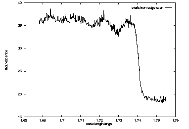
Figure 1a
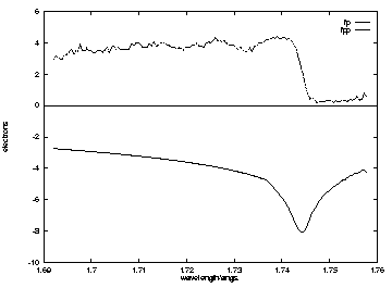
Figure 1b
Figure 1.a) The fluoresence XANES spectrum recorded from a single
crystal of desulphoredoxin using a single wire proportional counter on station
9.5 at Datesbury.
b) The transformed spectrum showing the values of f' and f'' in
electrons as a function of incident x-ray wavelength
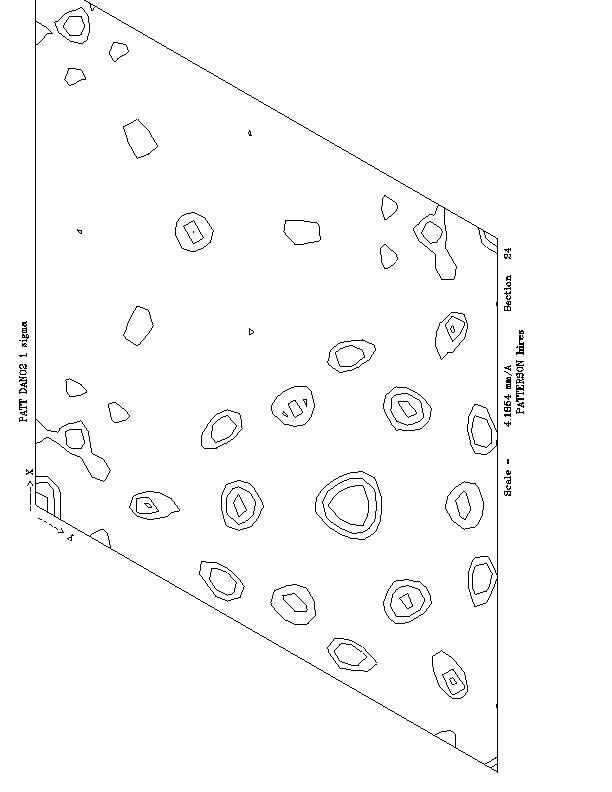
Figure 2a
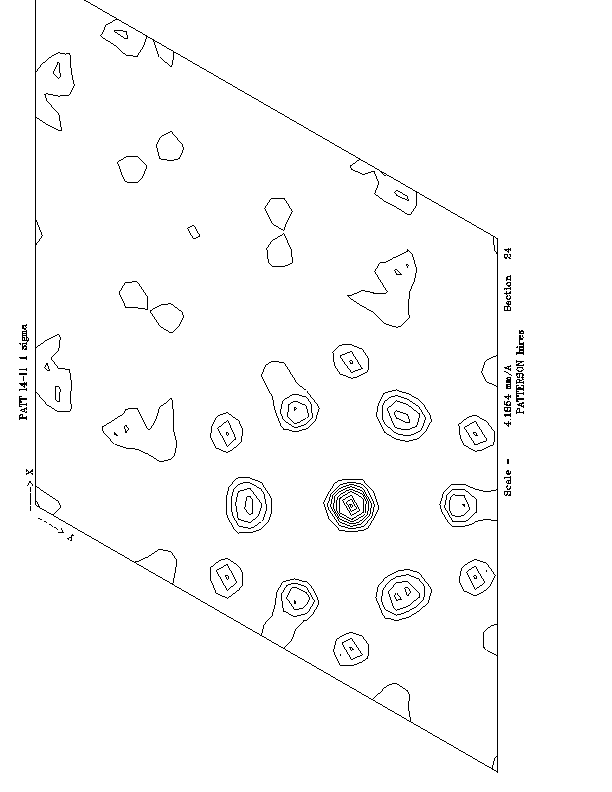
Figure 2b
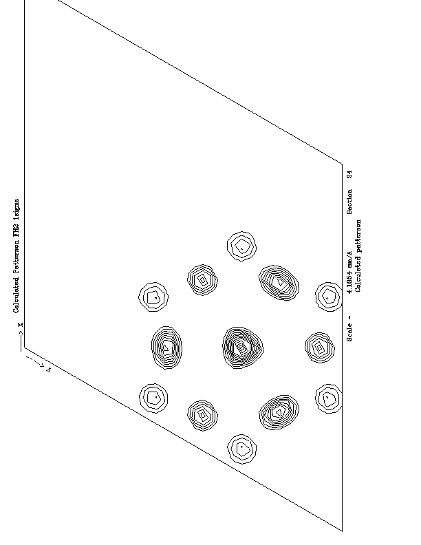
Figure 2c
Figure 2. a) Anomalous difference Patterson map calculated using the 2
(maximised f'') dataset, b) Dispersive difference Patterson calculated
using the difference in tructure factors between
1
and 4 c)
Calculated
Patterson map using refined Fe site positions.

Figure 3. The calculetd electron density map, showing 1/6th of the unit
cell in c the section direction, two unit cells in each other direction.