Table 1: Flowchart of general procedure
MAD is an extremely demanding technique which can yield good phases from high quality crystals and data. However, in combination with DM, usable maps can be obtained from datasets which are little better than average. The present work is intended to show that provided some care is taken in the early stages of the process, it is a straightforward technique which is of particular applicability to oligonucleotide crystallography.
Here I concentrate on the aspects of the technique as I have applied it, treating the problem as a variation on MIR using MLPHARE for heavy atom refinement.
The data for the three structures discussed here were all collected at the new synchrotron in Trieste, Italy, on the protein crystallography beamline 5.2R on visits in February and May 1996; they were the first three MAD datasets that I collected, and among the first to be collected at Elettra.
The beamline at Trieste is well suited to MAD because of the easily tunable X-ray source from ~0.62Å to ~3.1Å [1]. It supplies 1012 to 1013 monochromatic photons per second; although the X-rays are not quite as well focussed as at the ESRF, it is still an extremely bright source, and the reliability and stability are very high.
It is necessary to process the diffraction data as well as possible; small errors can lead to failure of MAD-DM as it uses extremely small differences between Bijvoet pairs, which are expected to be only slightly larger than the errors in the data themselves. Without concentrating on the data processing here, it should nevertheless be remembered that any outliers flagged in the output from scaling should be noted and if the deviations are particularly large, these reflections should be omitted manually from further processing, at least until the heavy atoms have been located; Patterson maps in particular are very sensitive to the presence of rogue reflections. The SCALEIT statistics for the merging R factors of and between datasets should also be examined; if the differences between the datasets are all about the same, then location of heavy atoms is unlikely to be successful by any means.
The majority of the calculations performed in these analyses were carried out with standard CCP4 [2] programs; the data for the first example have been made available as part of a worked example on the CCP4 server. Data reduction from raw images was carried out with Denzo and Scalepack [3] ; processing with other programs (e.g.MOSFLM and SCALA) will yield data of similar quality. The general scheme followed is outlined in Table 1.
Oligonucleotides are often available in much lower quantities than proteins, and this is eqspecially true of those species containing anomalous scatterers; also, crystallization is often difficult and thus few crystals are available. However, the monomer nucleotides or even nucleosides are available pure in large quantities, so in these experiments the XRF spectra were obtained for 5-bromo-2'-deoxyuridine and used to determine the appropriate wavelengths for data collection. The chemical environment of the bromine in 5-bromo-2'-deoxyuridine (the nucleoside) is very similar to that in 5-bromo-uracil (the free base) or even in an oligonucleotide containing 5-bromo-2'-deoxyuridine-5'-phosphate, hence XRF spectra obtained from these species are all extremely similar, and in general similar to that in Mark Peterson's in this Report.
Table 1: Flowchart of general procedure
The most important point is that the crystals containing the anomalous scatterer must be of high quality. Small crystals help avoid problems due to absorption; as the DFs are very small, a poor absorption correction could mask completely any effect being exploited.
At the synchrotron, the quality of the optics is paramount; it is essential that not only is the wavelength what you think it is, but also that it can be reliably and repeatedly reselected. The X-rays must be stable for extended periods, both in terms of intensity and wavelength. Small variations can easily accumulate into significant errors.
The advent of cryo-cooling of macromolecular crystals is one of the features that has made MAD-DM data collection reasonably straightforward recently. The ability to collect several complete datasets on a single crystal has increased the chance of success of this method considerably.
Many crystallographers make life more difficult for themselves by not trying the 'oil drop' technique, but instead search for cryoprotectants that may well contribute to increased mosaicity and reduction in data quality. Much of the degradation in crystal quality on freezing is due to surface moisture freezing rather than ice formation in the solvent channels inside the crystal [4] . The oil drop method, because it removes this surface moisture, will in many cases prevent crystal damage; it has never failed for me on either DNA or protein crystals. It has the added advantage that the crystal is coated in a hydrophobic layer, so it does not dry out and can be handled for some minutes outside its sitting or hanging drop.
I prefer to mount the crystal in a random orientation; this is advantageous in that the completeness of the datasets is increased over that obtainable from an aligned crystal. With a stable crystal and stable X-rays, there is little to be gained from the careful alignment of the crystal on an axis. The advantage of measuring Bijvoet pairs close together in time seems to be relatively unimportant, in DNA crystallography at least.
Atomic coordinates for the anomalous scatterers in each example were determined using the direct methods option in SHELXS-96 [5] (F2 data from Scalepack were processed with SHELX-PRO [6] to yield anomalous DF values). An example of the results of this strategy for the first sample is in Table 2; it can be seen that this route should be considered as the first choice for heavy atom determination. Direct Methods seem to be more 'robust', and resistant to the presence of outliers in the data than the Patterson method, and give answers in negligible time.
The reliability of direct methods can be judged from several criteria; chief amongst these in my view is that if the same results are obtained from each of the datasets with an anomalous contribution but not from the long wavelength offset, the answer is probably correct. Once (if!) they have failed it may be necessary to calculate Patterson maps, plot Harker sections and interpret these, but in the general case this will not be necessary. In my eagerness to look at electron density, I tend to glance over the SCALEIT statistics while the program output is scrolling past on screen, and only return to it later if difficulties have arisen.
MAD by itself will rarely provide enough phase information to be able to produce interpretable electron density maps; some kind of additional phase extension is usually required in addition. We have used the CCP4 program DM, which applies solvent flattening and histogram matching to the data, and this leads to maps which can be of very high quality.
A crystal of the cyclic DNA octamer CAT-BrU-CAT-BrU, which has the 5' and 3' ends joined, was used in this study.
Four datasets were collected , one each at a long wavelength offset, at the inflexion point, the white-line maximum and a short wavelength offset (Table 3). Processing of these data showed that they were reasonably complete, and using Scalepack's 'linear R-factor' and 'square R-factor' as guides, they were of reasonable but not exceptional quality.
Direct methods gave two possible bromine positions (see Table 2), which was expected from the unit cell dimensions and space group.
Heavy atom refinement according to the scheme in Table 1 gave the results in Table 4. It is worth spending a little time looking at the various figure of quality produced. For the Figures of Merit, values greater than 0.6 can be considered encouraging, and if > 0.8, the problem can be considered well on the way to being solved. The Cullis R-factors, which are calculated for each derivative should become smaller for a correct answer; final values of RCull(cen) < 0.9 and RCull(acen) < 0.6 for the white-line maximum and short wavelength offset datasets should be seen as encouraging, and an Rcull(ano) < 0.5 for the datasets with an anomalous contribution seems a good indicator that the correct answer is being approached
Another measure of the correctness of the refinement process can be found by inspection of the refined values of Occ and AOcc (the real and anomalous occupancies), as they should be proportional to delta-f' and f" respectively; even in the best collected datasets, there will be deviations from these relationships which reflect the fact that datasets have not been collected exactly at the inflexion point and whiteline maximum (Table 5). However, as long as the proportions are roughly correct, it is important not to worry too much.
|
| |
The main thing to be remembered about the various measures of quality associated with heavy atom refinement is that they are only guides; the best, and only sure way of knowing that the MAD-DM process has been successful is when calculated electron density is studied and model fitting can begin.
DM was run in a more-or-less default mode of solvent flattening with histogram matching; the only required information from the crystallographer is a reasonable estimate of the solvent fraction of the unit cell. The figure that seems most informative from DM is the Real Space Free R; this can give good information on the correct hand of the structure (which cannot be obtained from MLPHARE), and is also a further indication that the whole process has worked. Note that it is only after processing with DM that there is a significant difference between the two hands, and it is apparent in this case that originally the wrong hand was chosen. Phases are also calculated for many reflections unphased in previous steps, and this phase extension is important in being able to calculate electron density.
The phases calculated by DM can be used directly by FFT to produce an F(obs) map which can be viewed on a graphics workstation after suitable translation.
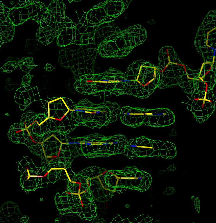
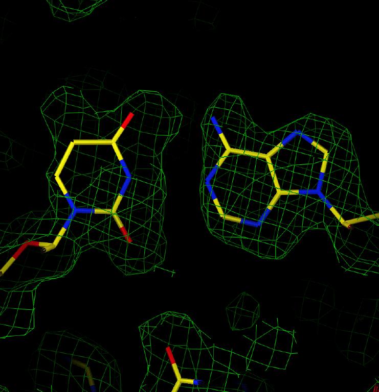
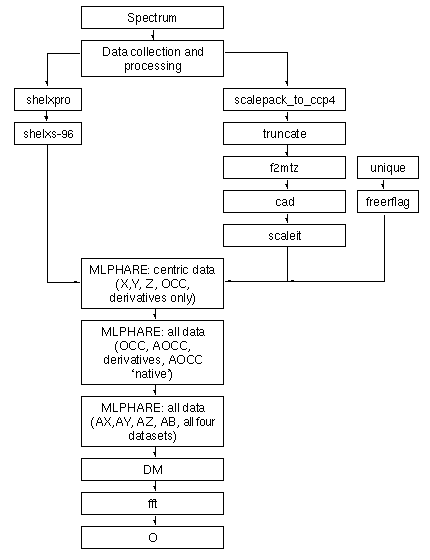
Figure 1: Electron density for sample 1 showing obvious base stacking. Figure 2: Electron density for sample 1 in the region of an A-T base pair.
The second sample was isomorphous with the native structure solved elsewhere. In this case, instead of four datasets, seven were collected; the extra three were collected with wavelengths at -1eV (#5), +1eV (#6) and +2eV (#7) from the measured inflexion point of the nucleotide. This experiment was intended to ensure that we had a dataset as close as possible to the true inflexion point of the oligonucleotide. As it turned out, the real value was between the measured IP and #5.
|
| | ||||||||||||||||||||||||||||||||||||||||||||||||||||||||||||||||||||||||||||||
The data collected were not of the same quality as for Crystal 1 (Table 2), but Direct Methods revealed the presence of four heavy atoms in the asymmetric unit, with roughly the same coordinates as those for the four non-base-paired thymine methyl groups in the native.
Examination of an F(obs) map in the region of an A-T base pair (Figure 3) reveals that the electron density is interpretable, but less easily than for sample 1. However, with some work the molecule could be successfully fitted even without prior knowledge of the correct structure.
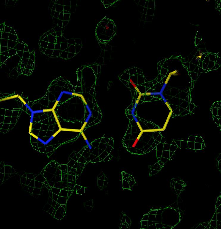
Figure 3: F(obs) electron density map in the region of an AT base pair for Sample 2.
This work is part of an ongoing project led by Dr Christine Cardin of Reading University, and I was in the fortunate position of helping her in this study. The crystal used was grown by Dr Adrienne Adams of Trinity College, Dublin.
The whole analysis from raw images to first electron density map took about one and a half working days, and only took that long because we took our time over it!.
The data collected appeared comparable at all stages of the processing to those from sample 1.
Direct methods found one heavy atom in the asymmetric unit. Heavy atom refinement proceeded smoothly, and examination of the measures of quality from DM show that there is little to choose between the correct and incorrect hand for this structure. However, note that the Real Space Rfree values for both hands are far worse than for the previous two samples; this should emphasize the point that all the numbers output by the programs should only be taken as guides!.
Electron density in an F(obs) map revealed that the solution from DM with the worse statistics was actually correct. Figure 4 shows the spectactularly good density for the oligonucleotide revealed in the first map calculated; it is not necessary to include a model of the structure to see in Figure 5 the positions of the Br in a BrU-A base pair and most of the base atoms as well.
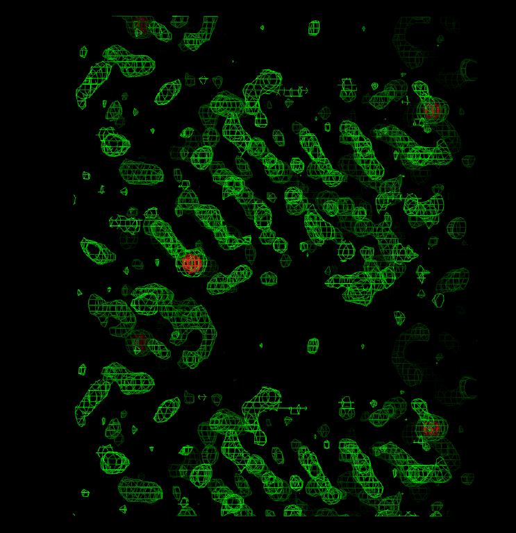
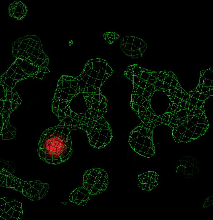
Figure 4: Electron density for sample 3 showing the base stacking. Figure 5: Electron density for sample 3 in the region of an A-BrU base pair. The density corresponding to the bromine atom is highlighted in red in each figure.
|
| | ||||||||||||||||||||||||||||||||||||||||||||||||
The take-home message from this work is that the facilities to collect data for a MAD-DM experiment and the programs to process these data are available now. MAD-DM is straightforward provided that data are collected carefully from the best available crystals; it is capable of giving excellent electron density which allows rapid and relatively easy structure building. The comparison of F(obs) maps for crystals 1 and 3 shows that it is necessary to examine the electron density rather than rely on the statistics; there can be a marked difference even between apparently similar data.
I wish to express my sincere gratitude to the following people and organizations; Eleanor Dodson (York), who guided me through the process of actually getting the phases and improving them; Christine Cardin, Alan Todd (Reading) and Adrienne Adams (Dublin), who provided the ideas and the crystal for sample 3 and much of the labour involved in collecting the data on all three crystals; Stephen Salisbury and Sarah Wilson (CCDC) who provided samples 1 and 2 and also spent sleepless nights at Elettra; the CCDC (for my salary!); University Library, Cambridge (for giving me time off to come to York for this meeting); especially to all the staff at Elettra, who have made collecting data there such a rewarding and interesting experience.
[1] see the WWW page http://www.elettra.trieste.it
[2] Collaborative Computational Project Number 4. 1994. "The CCP4 Suite: Programs for Protein Crystallography", Acta Cryst. D50, 760 - 763."
[3] Z. Otwinowski, Denzo and Scalepack, film processing programs for macromolecular crystallography. Yale University, New Haven, 1995.
[4] see, for example, http://www-structure.llnl.gov/Xray/cryo-notes/Cryonotes.html
[5] SHELXS-96, G.M.Sheldrick, Universität Göttingen, 1996
[6] SHELXPRO, G.M.Sheldrick, Universität Göttingen, 1996