 undulator on
the ESRF are given in table 3, assuming the source is demagnified to a 150
um image. A typical sample mosaicity (after freezing) may be
0.3o (5 mrad). The divergence of the beam at focal spot should
ideally be less than this.
undulator on
the ESRF are given in table 3, assuming the source is demagnified to a 150
um image. A typical sample mosaicity (after freezing) may be
0.3o (5 mrad). The divergence of the beam at focal spot should
ideally be less than this.
A. Thompson
EMBL Grenoble Outstation
The method of Multiple Wavelength Anomalous Diffraction [MAD] has been developed extensively in recent years by Hendrickson [1], Fourme [2] and Smith [3]. Small variations in intensity of diffraction spots due to resonant scattering of a heavy atom excited by the frequency of the incoming X-rays can be used in order to solve the crystallographic phase problem. The techniques and physics involved are described in the above reviews. The method is best pursued using the variable wavelength of radiation available at synchrotron sources, although in cases where the anomalous scattering is strong with respect to the size of the molecule allied techniques may be used on rotating anode sources ([4],[5] and [6]).
The "anomalous" intensity changes produced in the diffraction patterns are typically of the order of a few percent, and are (unfortunately) of a similar size to the errors (random and systematic) in good data! The methods of designing a beamline to maximise the chance of being able to collect MAD data by being aware of where error may creep into measurements are discussed in conjunction with the design of the MAD beamline (BM14) at the ESRF, its advantages and drawbacks.
It is very important to appreciate that a synchrotron beamline (whether for protein crystallography or anything else) is a single instrument designed for a specific function or type of measurement. The more flexible the beamline, the more compromises are likely to have been made in its design! Moreover almost any decision about a beamline parameter affects all the rest. For example if you require to study extremely small crystals and the X-ray source size is large compared to the crystal, substantial source demagnification (and hence increased divergence through the sample) may be required. This will have a knock on effect on the type of 2-D detector required - a large detector set far away from the sample would not necessarily be a good choice because of the increased divergence of the beam after the sample.
Beamline optimisation should then be discussed in terms of the source, optics, sample environment and detector, although I will discuss only the first two. The requirements of MAD will be discussed in the light of each of these. For a rigorous and well thought out discussion of beamline design, see Nave [7].
Some General Principles
Basically 3 types of source are available at modern synchrotrons - bending magnets (dipoles) or one of two insertion devices (wigglers or undulators). Their properties have been extensively discussed elsewhere. Table 1 gives several typical properties of these devices based on the ESRF source. The vertical and horizontal source size and divergences are matched to the sample size and mosaicity via conditioning optics. To achieve a narrow monochromatic bandpass with maximal flux, the divergence of the synchrotron beam in the dispersive direction must be matched to the natural monochromator bandpass.
MAD experiments have been reported at various absorption edges between the U Mv edge, 3.482 Å [8] and the Xe K edge, 0.358 Å [9]. Table 2 gives a copy of the periodic table showing absorption edges which may in principle at least be used - almost all of them! The source should be tunable between these limits, therefore. Some devices on 4th generation synchrotrons (bending magnets, wigglers) fulfil this requirement easily. Undulators, however, give a high peak brilliance in a narrow energy range (figure 1) with several harmonics of this energy, and therefore have to be tuned to give optimal intensity for a 3 wavelength MAD experiment. In this case, ÒtuningÓ refers to changing the gap between the permanent magnets in order to change the field and shift the energy spectrum. Wiggler and bending magnet sources are, by their nature, smoother, and hence require no "tuning" over the above wavelength range.
The above tuning of the undulator gap can perturb the electron beam position in the storage ring if the undulator field is not sufficiently symmetric (due to errors in construction or the increasing distortion of its frame due to the increasing magnetic field). Undulator "shimming" techniques developed at the ESRF have now improved to such an extent that this field inquality is much reduced and "tuning" is routinely possible L10]. In addition, shorter wavelength experiments which will need much tighter gap setting (for example for a MAD experiment at the Xe edge using the 5th harmonic of a "typical" undulator, a gap of 17 mm would be required) will soon be possible at the ESRF [11] and [12]). It is worth noting, however that a beamline optic that is optimised for 0.35 Å will not necessarily be optimised for 3.5 Å! In other words multiple lines may be needed to cover the whole wavelength range.
The source characteristics should be matched to the sample. Nowadays a
"typical" crystal seems to be more like 150 um than 300
um on edge. Source sizes and the corresponding convergence angles for a
bending magnet, wiggler and high and low
undulator on
the ESRF are given in table 3, assuming the source is demagnified to a 150
um image. A typical sample mosaicity (after freezing) may be
0.3o (5 mrad). The divergence of the beam at focal spot should
ideally be less than this.
A drifting wavelength causes different values of f' and f" to be "mixed" together, whereas a drifting intensity causes errors in inter filmpack scaling. The stability required depends on the actual bandpass chosen and the type of experiment performed. On BM14, the bandpass has been measured to be 2.4 x 10⁻⁴ from an Si (111) monochromator. For the anomalous signal to vary only 5% during the experiment with this bandpass and a wavelength of 1 Å, the energy must be stable to 0.2 eV over the period of the experiment. An energy stability of 0.5 eV rms can thus be regarded as good enough for all practical purposes, and this is easily within the measured source stability of the ESRF.
The beamline optics can also contribute to beam instability by heating, vibration or other obscure effects! The source power should thus not exceed practical limits of what modern (cooled) optics can tolerate. Typical power densities at 30m from the ESRF source with a single section insertion device (up to 3 possible) and 100 mA stored beam followed by the power ACTUALLY USED in recording a diffraction pattern (assuming 2.5 x 10⁻⁴ bandpass) are given in Table 4 [13] Many papers have been written on high power beam optics, and several successful approaches are available for both undulator and wiggler beams. Even so, when the requirement is for stability, reproducibility and reliability, it seems logical to use the most efficient source available, ie the undulators.
This has to be adequate to perform the experiment in a "reasonable" period of time, both from the point of view of getting good data ("systematic errors" can be time dependent, and sufficient couting time per image has to be spent to have adequate statistics) and getting your experiment scheduled when there is so much pressure on synchrotron beamlines! At the ESRF (even on the bending magnet beamline) the detector readout time is almost always longer than the required exposure time (for image plate detectors). The overall source intensity chosen therefore depends only on the thermal properties of the beam (see above) and the capacity of the sample to withstand the beam.
Required Wavelength Resolution
What is the appropriate energy bandpass for MAD experiments? These limits are
defined by the fineness of the sharpest features ("white lines")
in your absorption spectrum. Krause and Oliver [14] tabulate the I; and L level
X-ray line widths for Z from 1 to 110 . The widths result from the lifetime of
excited states, limited by the uncertainty principle
 "White line" effects (Lye et al [15], Brown et al [16] and Lytle
et al [17]) are present in L "edges" (where a transition from a
core level to one of a high possible density of final states gives the
"amplified" nature of the feature) or K edges (which may be due to different
transitions to exciton levels). The line widths of some L edge white lines have
been reported by Arp et al [18] and are in close agreement with the above
tabulated values for Z
"White line" effects (Lye et al [15], Brown et al [16] and Lytle
et al [17]) are present in L "edges" (where a transition from a
core level to one of a high possible density of final states gives the
"amplified" nature of the feature) or K edges (which may be due to different
transitions to exciton levels). The line widths of some L edge white lines have
been reported by Arp et al [18] and are in close agreement with the above
tabulated values for Z  50. Hence the required energy bandpass
for a MAD beamline should be such that the instrument broadening due to the
monochromator bandpass, vibration etc do not obscure the natural widths of
features on the absorption edges. Table 5 gives (in percent) the ratio between
the "core-hole" lifetime as given in [14] and energy of the X-ray absorption
edge. Features are broadened by the convolution of the instrument resolution
and the width of the feature. In the case of the fine Se absorption edge, a
bandpass of 1 x 10⁻⁴ would give effectively no broadening. It can be
inferred that a bandpass lower than around 1.0 x 10⁻⁴ will limit
intensity without making features significantly sharper. However it is also
clear that in some cases (for example Hg) such a narrow bandpass will give no
useful increase in anomalous signal. It may be then useful to have a facility
with a changeable bandpass between 1.0 x 10⁻⁴ and 3.0 x
10-4 such as could be achieved, for example, by an interchangeable
pair of Si (111) and Si(311) monochromators such as are available on BM14
(allowing for increased bandpass due to the intrinsic Si quality, surface
finish etc).
50. Hence the required energy bandpass
for a MAD beamline should be such that the instrument broadening due to the
monochromator bandpass, vibration etc do not obscure the natural widths of
features on the absorption edges. Table 5 gives (in percent) the ratio between
the "core-hole" lifetime as given in [14] and energy of the X-ray absorption
edge. Features are broadened by the convolution of the instrument resolution
and the width of the feature. In the case of the fine Se absorption edge, a
bandpass of 1 x 10⁻⁴ would give effectively no broadening. It can be
inferred that a bandpass lower than around 1.0 x 10⁻⁴ will limit
intensity without making features significantly sharper. However it is also
clear that in some cases (for example Hg) such a narrow bandpass will give no
useful increase in anomalous signal. It may be then useful to have a facility
with a changeable bandpass between 1.0 x 10⁻⁴ and 3.0 x
10-4 such as could be achieved, for example, by an interchangeable
pair of Si (111) and Si(311) monochromators such as are available on BM14
(allowing for increased bandpass due to the intrinsic Si quality, surface
finish etc).
The combination of a vertical focussing mirror and a horizontal focussing triangular monochromator as described in [19] is one of the most commonly used optics for synchrotron radiation. This geometry can be used for MAD measurements where the beamline bandpass (Emitted by the monochromator bandpass and beam horizontal divergence) is small enough, for example in [10]. It offers several important advantages:
* Can focus a large horizontal acceptance, depending on the exact geometry.
* Angle of monochromator, sample and collimation defines wavelength therefore changes in machine vertical and horizontal orbit or mirror vibration cause only intensity (not wavelength) changes.
* Easy to get fine focal spot - Si or Be give adequate bandpass.
* Permits "Simultaneous" MAD [20] if used with a large crossfire angle and hence bandpass, but can be used for ordinary MAD [10] with a narrow bandpass monochromator and pencil beam.
On the other hand the system has the following disadvantages:
* A nuisance to change wavelength, and hard to make wavelength change reproducible (need to move monochromator and sample and detector).
* Crossfire from the focussing - either the beamline is very long, or has a large defocussing ratio.
A more recent approach to a MAD beamline is evidenced by SRS 9.5 [21] which uses a toroidal mirror and channel cut monochromator to provide a beam whose position changes very little with wavelength, and a tight focus. This very simple optic has two major disadvantages :
* Need to limit vertical aperture (and hence intensity) to get a narrow energy bandpass.
* Small horizontal acceptance (less than 2 mrad).
It is interesting to note that both these disadvantages are almost eliminated with the narrow vertical and horizontal divergences of an undulator source.
Of course there are many variations on the theme of focussing beam with narrow bandpass and constant focal spot position with wavelength, for example the extremely successful Howard Hughes Medical Institute line at Brookhaven [22] which uses a horizontally focussing constant height monochromator and a vertically focussing mirror.
The ESRF beamline D2AM [23] uses a similar horizontal focussing monochromator, sandwiched between two X-ray mirrors. The first of these collimates the incoming radiation in the vertical ie there is (almost) no beam divergence component to the energy bandpass of the monochromator. The monochromatic beam is subsequently focussed by the second mirror.
The horizontally focussing monochromator arrangement has two main disadvantages in producing a fine focal spot -
* Its main advantage lies in focussing large horizontal divergences. However unless the surface shape of the monochromator can be made conical rather than cylindrical, it has to be used close to a 3:1 demagnifying configuration to give maximum throughput into the narrow bandpass [24]. This demagnifying ratio causes significant beam crossfire and hence reduces the unit cell size resolvable for a given detector.
* The bending radius has to be continually changed with energy in order to keep a tight focal spot (and hence stable intensity with wavelength variation on the sample). In fact the change in intensity over a typical experimental energy range can be large [25,26].
The approach adopted on ESRF beamline BM14 is a combination of the above approaches, with a collimating mirror, channel cut monochromator and a vertical and horizontal focussing mirror. The great disadvantage of this system are the optical aberrations due to the double mirror arrangement (the so called "slope error" contributes twice to the vertical broadening of the focal spot) and the differing object and image distances for the vertical (source at "infinity" as the beam is collimated) and horizontal (source at "source" position) foci. This latter effect is in practise very small for a narrow horizontal beam acceptance and small mirror grazing angle. A recent scheme for the proposed British Beamline at the ESRF [25] suggested using parabaloidal mirrors to limit this aberration.
Other geometries exist, for example the novel trichromator [27] principle proposed for the RIKEN beamline on SPRING-8. The success of this approach is for the future to reveal!
The beamline BM14 was designed to give a high stability beam with maximum intensity into a narrow wavelength bandpass.
* Wavelength Range 0.6 - 1.8 Å
* Intensity approximately 2.5 x 10¹² photons per second at 1 Å wavelength into a focal spot of 0.8 mm x 0.3 mm.
* Rapid tunability - a few minutes to scan the whole wavelength range.
* Wavelength stability 0.1 eV rms.
* Intensity stability 0.8 % rms.
* Fast readout detectors (Offline FUJI plate, CCD and MAR 345)
To date a fifteen new structures have been solved on BM14 by MAD phasing, with several others in various stages of data analysis. Amongst these the weakest anomalous signal was 2.5%, and a typical signal is more like 3.5%. (Data quality (and hence crystal quality) has to be extremely good to use signals below 3% for MAD).
Beam intensity and wavelength stability can be good enough to collect data from stable (cryo- cooled) crystals in a random orientation, and a substantial fraction of the successful MAD phasing experiments on BM14 have been performed in this way. Care must of course be taken in order to record complete data including all measurements of Bijvoets, and to have a large redundancy of measurement. Inverse beam data collection or setting of a crystal around a mirror plane are preferable when searching for an extremely small signal, with an unstable beam or with uncooled crystals. A typical experiment on BM14 takes between 24 and 48 hours, depending on whether image plate or CCD detector is used.
The largest number of anomalous scatterers (that I am aware of) used in ab initio MAD phasing was 12 (a bacterial synthetase on the French ESRF Beamline D2AM by Fanchon and Bertrand). Examples of 6-10 anomalous scatterers are relatively common (for example Matias [28], Ceska [29]). Larger structures (J. A. Smith) have been shown to give good phases based on already refined Se signals, and direct methods has been used to identify 18 out of 22 Se sites in the asymmetric unit from a MAD data set collected on BM14 [30]
Recently some attention has been paid to the advantages of measuring phases to very high resolution [31], the ability to do this without worries of lack of isomorphism being one of the major advantages of MAD.
Interest is now being focussed on undulator beamlines for MAD protein crystallography (Westbrook(APS), Thompson et al [32], Shapiro et al [10]), where smaller crystals can be studied, or higher resolution data should be improved due to the improved beam collimation. Data collection times will become much smaller, and with rapid readout CCD detectors, fine phi oscillations will improve data quality due to the improved background per reflection. Finally, with extensive work by Schiltz et al [33] and increasing interest in soft "M" absorption edges, MAD will soon be extended to new wavelength ranges.
* MAD is a routine technique on modern beamlines, and many technical problems have solved (only to reveal subtle new ones!)
* An undulator is the best currently available source for a MAD beamline.
* Several optics solutions exist which should be well adapted to an undulator source.
Although the comments in the above paper are by me, the success of BM14 is due to the work of many people, namely :
V. Biou (IBS Grenoble), G. Blattman (ESR.F), L. Claustre (EMBL Grenoble), A. Gonzalez (EMBL Hamburg), S. Laboure, G. Leonard, G. Marot and M. Mattenet (ESRF), V. Stojanoff and O Svensson (ESRF) and P. Thorander (Siemens).
1. Wayne A Hendrickson. Science 254 (1991) pp 51- 58.
2. Roger Fourme, William Shepard and R.ichard Kahn. Progress in Biophysics and Molecular Biology 64 (1996) pp 167 - 199.
3. Janet L. Smith. Current Opinion in Structural Biology 1 (1991) pp 1002 - 1011.
4. Wayne A Hendrickson and Martha M Teeter. Nature 290 (1981) pp 107 - 113.
5. S-E Ryu, P D Kwong, A Truneh, T G Porter, J Arthos, M Rosenberg, X Dai, N Xuong, R Axel, R W Sweet and W A Hendrickson. Nature 348 (1990) pp 419 - 426.
6. Mariusz Jaskolski and Alexander Wlodawer. Acta Crystallographica D52 (1996) pp 1075 - 1081.
7. Colin Nave. In preparation.
8. Hendrickson, personal communication.
9. Roger Fourme, personal communication.
10. L. Shapiro, A. Fannon, P. Kwong, A. Thompson, M. Lehmann, G. Grubel, J-F. Legrand, J Als-Nielsen, D. Colman and W. Hendrickson. Nature 374 (1995) pp 327 - 337.
11. ESRF Internal Memo, Ropert (1996).
12. ESRF Annual Report (1995) p 103.
13. ESRF ÒRed BookÓ (1991).
14. M. O. Krause and J. H. Oliver. Journal of Physical and Chemical Reference Data 8 no. 2 (1979) pp 329 - 338.
15. Richard C. Lye, James C. Phillips D. Kaplan, S. Donaich and Keith O. Hodgson. Proceeding of the National Academy of Science (USA) 77 (1980) pp 5883 - 5888.
16. M. Brown, R. E. Peierls and E. A. Stern. Physical Review B 15 (1977) pp 738 - 744.
17. F. W. Lytle, P.S.P. Wei, R. B. Greegor, G. H. Via and J. H. Sinfelt. Journal of Chemical Physics 70 (1979) pp 4849 - 4855.
18. U. Arp, G. Materlik, M. Meyer, M. Richter and B. Sonntage. in X-Ray Absorption Fine Structure. Edited by S S Hasnain (1991) pp 44 - 47.
19. M. Lemmonier, R. Fourme, F. Rousseaux and R. Kahn. Nuclear Instruments and Methods 152 (1978) pp 173 - 177.
20. Lee and C. Ogata. Journal of Applied Crystallography 28 (1995) pp 661 - 665.
21. A. Thompson, J. Habash, S Harrop, .J. R. Helliwell, C. Nave, P. Atkinson, S. S. Hasnain, I. D. Glover, P. R. Moore, N. Harris, S. Kinder and S. Buffey. Review of Scientific Instruments 63 (1992) pp 1062 - 1064.
22. J-L. Staudenmann, W. Hendrickson and Abramowitz. Review of Scientific Instruments 60 (1989) pp 1939 - l942.
23. J-P. Simon, E. Geissler. A-M. Hecht, F. Bley, F. Livet, M. Roth, J-L. Ferrer, E. Fanchon, C. Cohen-Addad, J-C Thierry. Review of Scientific Instruments 63 (1992) pp 1051 - 1054.
24. C. Sparks, Borie and J. Hastings. Nuclear Instruments and Methods 172 (1980) pp 237- 242.
25. D. Paul, M. Cooper and W. Stirling. Review of Scientific Instruments 66 no. 2 (1995) pp 1741 - 1744.
26. A. Thompson and . Kvick. Report to the ESRF Scientific Advisory Committee (1992).
27. M. Yamamoto, T. Fujisawa, M. Nagasako, T. Tanaka, T. Uruga, H. Kimura, H. Yamaoka, Y. Inoue, H. Iwasaki, T. Ishikawa, H. Kitamura and T. Ueki. Review of Scientific Instruments 66 no. 2 (1995) pp 1833 - 1835.
28. P. Matias, J. Morais, A. Coelho, R. Meyjers, A. Gonzalez, A. Thompson, L. Sieker, J. LeGall and M-A. Carrondo in preparation.
29. T. A. Ceska, J. R. Sayers, G. Stier and D. Suck. Nature 382 (1996) pp 90 - 93.
30. J. A. Smith (personal communication) using software developed by Woolfson et al (RANTAN).
31. F.T. Burling, W.I. Weis, K.M. Flaherty and A.I. Brunger. Science 271 (1996) pp 72 - 77.
32. V. Biou, A. Gonzalez, J. Helliwell, S. McSweeney, J.A. Smith and A. Thompson (1995). Report to the ESRF Science Advisory Committee.
33. M. Schiltz. W. Shepard, R. Fourme, T. Prange, E. De la Fortelle and G. Bricogne. Acta Crystallographica D52 (1997) pp 78 - 92.
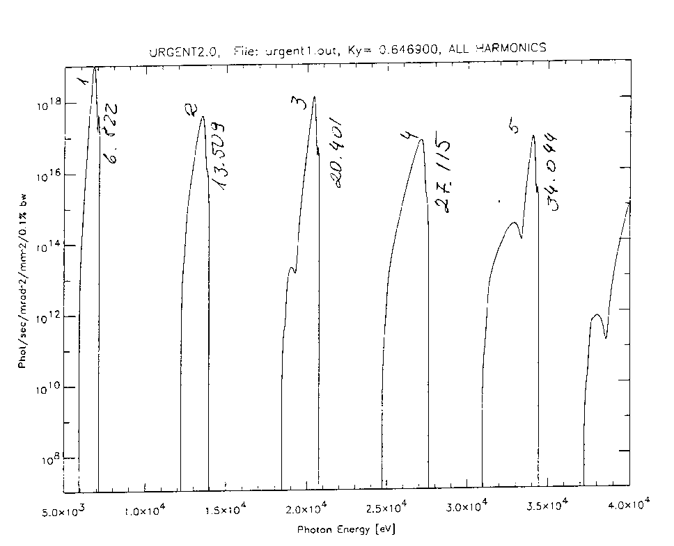
A calculated ESRF Undulator spectrum showing the discrete and narrow peaks of X-ray intensity. Brilliance is plotted against energy.
Table 1
                          ESRF Source Properties
                     At beam exit from the shield wall
                        Taken from ESRF "Red" Book
                          Storage Ring at 200 mA
           Power    Horiz Size mm  Vert Size mm   Power /        Power / area
           KW                                     length W/mm    W/mm**2
B.M.       0.84     126            2.3            6.7            2.9
Und.       2.4      5.5            3.3            495            149
Wigg.      14       52             3.3            252            76
Note on table 2:-
Normally the larger edge transitions are better for MAD ie an L edge gives a bigger signal than a K edge etc. For this reason only the L3 and M5 edges are quoted. The usefulness of the absorption edges also (on average) increaases with increasing Z. However the difficulty in collecting accurate data at long wavelengths (low energies) should be borne in mind when preferring, for example the Xe L3 edge to the K edge. Certain elements give "white lines" (for example Se) which "amplifies" the signal available. Where "white lines" occur for a K edge, they should also be present for L1. When they occur for L3 they should also be present for L2.
Key to table 2:-
11.111 Accessible for MAD on most beamlines
11.111 Accessible for MAD on some beamlines
11.111 Not accessible for MAD
* 11.111 * Already successfully used for MAD
* 11.111 * Of potential future interest for MAD
Energies are given in KeV
Periodic Table Showing Absorption Edges
Element           K             L3            M5
H                 0.016
He                0.025
Li                0.055
Be                0.112
B                 0.188
C                 0.284
N                 0.410
O                 0.543
F                 0.697
Ne                0.870
Na                1.071
Mg                1.303
Al                1.559
Si                1.839
P                 *2.149*
S                 *2.472*
Cl                2.833
Ar                3.206
K                 3.608
Ca                *4.039*
Sc                4.492
Ti                4.966
V                 5.465
Cr                5.989
Mn                6.539
Fe                *7.112*
Co                7.709
Ni                8.333
Cu                *8.979*
Zn                *9.659*
Ga                10.367
Ge                11.103
As                11.867
Se                *12.658*
Br                *13.474*
Kr                14.326
Rb                15.200
Sr                16.105
Y                 17.038
Zr                17.998        2.233
Nb                18.986        2.371
Mo                20.000        2.520
Tc                21.044        2.677
Ru                22.117        2.838
Rh                23.220        3.004
Pd                24.350        3/.173
Periodic Table Showing Absorption Edges
Element           K             L3            M5
Ag                25.514        3.351
Cd                26.711        3.538
In                27.940        3.730
Sn                29.200        3.929
Sb                30.491        4.132
Te                *31.814*      *4.341*
I                 *33.169*      *4.557*
Xe                *34.561*      *4.782*
Cs                35.985        5.012
Ba                              5.247
La                              5.483
Ce                              5.723
Pr                              5.964
Nd                              6.208
Pm                              6.459
Sm                              *6.716*
Eu                              6.977
Gd                              *7.243*
Tb                              7.514
Dy                              7.790
Ho                              *8.071*
Er                              8.358
Tm                              8.648
Yb                              *8.944*
Lu                              9.244
Hf                              9.561
Ta                              9.881
W                               *10.207*
Re                              10.535
Os                              *10.871*
Ir                              11.215
Pt                              *11.564*
Au                              *11.919*
Hg                              12.284        2.295
Tl                              12.658        2.485
Pb                              *13.055*      2.586
Bi                              13.419        2.580
Po                              13.814        2.683
At                              14.214        2.787
Rn                              14.619        2.892
Fr                              15.031        3.000
Ra                              15.444        3.105
Ac                              15.871        3.219
Th                              16.300        3.332
Pa                              16.733        3.442
U                               *17.166*      3.552
                Beam Size and Convergence of ESRF Straight Sections
Horiz size        Horiz Div         Horiz Conv        Vert Size         Vert Div
                               Low  Position
0.97              37.6              243               0.23              13.9
                               High  Position
0.11              197               145               0.47              15.5
                    All sizes in mm, divergences in urad, FWHM.
Table 4
            Power emitted by ÒtypicalÓ insertion devices
                  at the ESRF, 100mA stored current
Source                  Power Density 30m       Percentage Power Used
Bending Magnet          1.1                     0.0013
Undulator (high         20                      0.01
)
Wiggler                 20                      2 x 10⁻⁶
Table 5
Key to table 5:-
Energy of edge in KeV, width of absorption edge in eV, ÒWLÓ width is theÓwhite line widthÓ in eV.
             Theoretical Natural widths and measured values
                       of several absorption edges
Element       Edge          Width         Ratio             ÒWLÓ width
Fe            7.112         1.25          1.76 x 10⁻⁴
Se            12.658        2.33          1.84 x 10⁻⁴
Hg            14.209        5.5           3.87 x 10⁻⁴
Pt            13.273        5.86          4.41 x 10⁻⁴       5.2 x 10⁻⁴
Yb            8.944         5.14          4.6 x 10⁻⁴        4.5 x 10⁻⁴